Uncommon Ground

Population genetics

Sharing a new version of my genetic drift simulation

You may be aware that I wrote a series of applications in RShiny several years ago to illustrate some principles of population genetics. I just finished revising the genetic drift application. If you’ve used it in the past, you’ll know that it would get hung up when you tried to simulate a long time series or a lot of populations. After some digging around, I realized that the problem isn’t with running the simulation or with collecting the results. It’s with converting the results to a form that allows the simulation to unfold over time.

As a result, this version allows you to turn the animation off. Now you can run long time series with lots of populations (where “lots” equals “up to 10”). You won’t see the results played as a movie, but you’ll see them displayed very quickly. As you’ll see from the first link above, all of the source code is available on Github. If you find any of these applications useful, you’ll want to take a look at the Google Doc that Katie Lotterhos put together and announced on Twitter last January. It includes screenshots and links to applications written by CJ Battey, Graham Coop, and Chris Muir.

Genetic structure and clonal diversity in an important Chinese grass

Since you’re reading this blog, you must know that I don’t have a lot of time for research these days. My duties as Vice Provost for Graduate Education and Dean of The Graduate School at UConn take up most of my time. I do manage to contribute to some research, so long as other people do the real work and I contribute some ideas or some statistical analyses. Here’s another example of that.

Last fall I was asked about the old C++ program Hickory that I had written to facilitate analysis of Wright’s F-statistics with dominant markers. It was never terribly widely used, and it was difficult to maintain. I gave up about 10 years ago. In the meantime, I realized that there’s an easy way to rewrite Hickory using Stan. After being contacted, I finally bit the bullet and did the rewrite in a combination of Stan and R. I even mentioned the R/Stan implementation last September.

Yesterday, we posted a pre-print on bioRxiv that uses the new version of Hickory as one of a variety of analytical methods that provide some insight into the genetic structure of Leymus chinensis. Here’s the abstract and a link.

Genetic structure in patchy populations of a candidate foundation plant: a case study of Leymus chinensis (Poaceae) using genetic and clonal diversity

Jian Guo, Christina L. Richards, Kent E. Holsinger, Gordon A. Fox, Zhuo Zhang, Chan Zhou

doi: https://doi.org/10.1101/2021.06.12.448174

PREMISE The distribution of genetic diversity on the landscape has critical ecological and evolutionary implications. This may be especially the case on a local scale for foundation plant species since they create and define ecological communities, contributing disproportionately to ecosystem function.

METHODS We examined the distribution of genetic diversity and clones, which we defined first as unique multi-locus genotypes (MLG), and then by grouping similar MLGs into multi-locus lineages (MLL). We used 186 markers from inter-simple sequence repeats (ISSR) across 358 ramets from 13 patches of the foundation grass Leymus chinensis. We examined the relationship between genetic and clonal diversities, their variation with patch-size, and the effect of the number of markers used to evaluate genetic diversity and structure in this species.

RESULTS Every ramet had a unique MLG. Almost all patches consisted of individuals belonging to a single MLL. We confirmed this with a clustering algorithm to group related genotypes. The predominance of a single lineage within each patch could be the result of the accumulation of somatic mutations, limited dispersal, some sexual reproduction with partners mainly restricted to the same patch, or a combination of all three.

CONCLUSIONS We found strong genetic structure among patches of L. chinensis. Consistent with previous work on the species, the clustering of similar genotypes within patches suggests that clonal reproduction combined with somatic mutation, limited dispersal, and some degree of sexual reproduction among neighbors causes individuals within a patch to be more closely related than among patches.

An R-Stan implementation of Bayesian inference for Wright’s F-statistics

Some of you know that many years ago Paul Lewis, Dipak Dey, and I wrote a paper describing a Bayesian approach to inferring population structure from dominant markers.1 You may also know that Paul Lewis and I wrote a Windoze program in C++, Hickory, that implemented the approach. We later extended Hickory for analysis of co-dominant markers. Later still, Feng Guo, Dipak, and I wrote another paper describing a Bayesian approach to (a) estimating population- and locus-specific effects on FST and (b) identifying loci where the posterior distribution of FST is markedly different from the overall estimate.2 If you know that (and maybe even if you don’t know all of that), you also know that Paul and I stopped maintaining Hickory a number of years ago. I moved from Windoze to Mac, and the library we were using to support the graphical user interface became too complicated for me to keep up with.

I’ve had a few requests from people who were interested in using Hickory, but I just haven’t had the time to find a way to support them – until now.

Over the past several years, I’ve been using Stan for many different statistical analyses. When I received another request for Hickory a couple of weeks ago, I realized that I could pretty easily develop a new version of Hickory in R/Stan. This approach has several advantages over the standalone C++ code in the original Hickory.

  1. I don’t have to worry about writing the MCMC sampler myself. I use the very sophisticated Hamiltonian Monte Carlo in Stan. I not only avoid me the bother of writing my own sampler, I have much greater confidence that the sampler is performing correctly. It’s written and maintained by experts, and the convergence diagnostics are far more sophisticated than for Metropolis-Hastings.
  2. It should be readily portable to any platform on which R is supported. The only requirement, for now, is that you have a C++ compiler installed. If you’re running a Mac, you may need to download Xcode. If you’re running Linux, you should be all set. If your running Windows, you can download Rtools from CRAN. I intend to submit the R package I’ve written to CRAN once I’ve tested it more thoroughly and provided some extensions to the crude functionality currently available. Once it’s on CRAN, you won’t even need a C++ compiler.
  3. I can develop an interface to adegenet and other R packages used for analysis and manipulation of genetic data so that Hickory can use data in many different formats supported by other packages.

A very early release of Hickory is available at GitHub. You should find all of the information you need to install and use it there. Let me know if you run into problems. I’ll do my best to walk you through them (and probably correct some errors I’ve made or at least improve the meager documentation in the process).

  1. Holsinger, K. E., Lewis, P. O., and Dey, D. K. 2002. A Bayesian approach to inferring population structure from dominant markers. Molecular Ecology 11:1157–1164.
  2. Guo, F., Dey, D. K., and Holsinger, K. E. 2009. A Bayesian hierarchical model for analysis of SNP diversity in multilocus, multipopulation samples. Journal of the American Statistical Association 104:142–154. http://doi.org/10.1198/jasa.2009.0010

Making accessible HTML from LaTeX sources — an additional experiment

Last week I reported on my initial experiments using Pandoc and LaTeXML to convert LaTeX to HTML. Here are links to the PDF produced with pdfLaTeX and the HTML:

If you’re like me, you’ll prefer the LaTeXML version to the Pandoc version, but as I pointed out the LaTeXML version includes CSS to customize the styling and the Pandoc version doesn’t. I did a quick Google search, figured out how to add CSS (and a table of contents) to the HTML output from Pandoc, and found a very nice CSS style to use (from Pascal Hertlief on Github). It’s possible that I’ll fiddle with Pascal’s CSS a bit, but there’s a good chance I won’t change it at all. It makes the HTML look really, really nice:

What I haven’t tried yet is converting LaTeX source that includes PDF figures. Let’s try that now and see how it works.

It took a while to get ImageMagick installed, to write a short Perl script to change all of the references to EPS files into references to PNG files and convert the EPSs to PNGs, but I really like the results. But this gets two of my three “to-dos” out of the way.


  • Check CSS styling for Pandoc.
  • Show the results to an accessibility expert at UConn and get some feedback on the different approaches.
  • See what happens with figures when they’re included in a LaTeX document.

Now I just (just?) need to check with an accessibility expert to confirm that the HTML is accessible. If it is, I’m all set.

By the way, if you’re interested in seeing the Perl script, let me know. It will be posted in the Github archive where I post the LaTeX source for my notes later this fall, but I’d be happy to send you a copy now if you drop me a line.

Making accessible HTML from LaTeX sources – some initial impressions

Some of you know that I’ve been making notes from my graduate course in Population Genetics available online for nearly 20 years (http://darwin.eeb.uconn.edu/uncommon-ground/eeb348/notes/). What a smaller number of you know is that I use LaTeX to write my notes and pdfLaTeX to produce PDFs from the LaTeX source. So far as I can tell (using ANDI), the PDFs produced in this way provide some elements that aid accessibility, but I am exploring options to produce HTML from the same source that might produce documents that are accessible to more readers. For my first experiment, I used the LaTeX file from 2019 that produced notes on resemblance among relatives. Here are links to three versions of the notes:

Both approaches to producing HTML are straightforward.

For Pandoc:

pandoc --standalone --mathjax -o quant-resemblance-pandoc.html quant-resemblance.tex

For LaTeXML:

latexml --includestyles --dest=quant-resemblance.xml quant-resemblance.tex
latexmlpost --dest=quant-resemblance-latexml.html quant-resemblance.xml

With the default options, I like the look of the LaTeXML version better, but it also includes CSS customizations and the Pandoc version doesn’t. It’s probably possible to include customized CSS with Pandoc, but I haven’t had a chance to investigate that yet. I also haven’t had a chance to consult anyone who knows how to judge accessibility of documents. When I’ve had a chance to do that. I’ll return with a report. (Don’t hold your breath. I am a dean, so I don’t have a lot of time on my hands.)

Here’s my to-do list, so that I don’t forget:

  • Check CSS styling for Pandoc.
  • Show the results to an accessibility expert at UConn and get some feedback on the different approaches.
  • See what happens with figures when they’re included in a LaTeX document.

If you have additional questions, let me know, and I’ll add them to the list.

Lecture notes in population genetics – final version from Spring 2017

I’ve finally had time to clean and post the final version of lecture notes from my graduate course in population genetics last spring. The individual lectures have been since I revised them for class, meaning that the last set of them was available in late April. You will find links to the individual lecture notes at http://darwin.eeb.uconn.edu/uncommon-ground/eeb348/notes/. If you’re interested in a particular topic in population genetics and I have a lecture that covers the topic, that’s probably where you’ll want to go.

If you want a single-volume reference to population genetics (including some old notes that I no longer maintain), you’ll find a PDF (5.89MB, 322 pages) at Figshare (doi: 10.6084/m9.figshare.100687.v2). If you want to print the PDF, I recommend that you print it on a double-sided printer. You can then put the pages in a binder and flip through them as if it were a bound book.

If you use LaTeX (and you’re a glutton for punishment), the LaTeX source and EPS files (for figures) is available in a Github repository (https://kholsinger.github.io/Lecture-Notes-in-Population-Genetics/).

These notes are released under a Creative Commons Attribution-ShareAlike license (http://creativecommons.org/licenses/by-sa/4.0/). I hope you find them useful. If you find errors in them, please let me know.

Causes of genetic differentiation in Protea repens

American Journal of Botany Volume 104, Number 5. May 2017.

Protea repens is the most widespread member of the genus. It was one of the focal species in our recently completed Dimensions of Biodiversity project. Part of the project involved genotyping-by-sequencing analyses of 663 individuals from 19 populations spanning most of the geographical range of the species. We summarize results of those analyses in a paper that just appeared in advance of the May issue (cover photo featured above) of the American Journal of Botany. Here’s the abstract. You’ll find the citation and a link at the bottom.

PREMISE OF THE STUDY: The Cape Floristic Region (CFR) of South Africa is renowned for its botanical diversity, but the evolutionary origins of this diversity remain controversial. Both neutral and adaptive processes have been implicated in driving diversification, but population-level studies of plants in the CFR are rare. Here, we investigate the limits to gene flow and potential environmental drivers of selection in Protea repens L. (Proteaceae L.), a widespread CFR species.
METHODS: We sampled 19 populations across the range of P. repens and used genotyping by sequencing to identify 2066 polymorphic loci in 663 individuals. We used a Bayesian FST outlier analysis to identify single-nucleotide polymorphisms (SNPs) marking genomic regions that may be under selection; we used those SNPs to identify potential drivers of selection and excluded them from analyses of gene flow and genetic structure.
RESULTS: A pattern of isolation by distance suggested limited gene flow between nearby populations. The populations of P. repens fell naturally into two or three groupings, which corresponded to an east-west split. Differences in rainfall seasonality contributed to diversification in highly divergent loci, as do barriers to gene flow that have been identified in other species.
CONCLUSIONS: The strong pattern of isolation by distance is in contrast to the findings in the only other widespread species in the CFR that has been similarly studied, while the effects of rainfall seasonality are consistent with well-known patterns. Assessing the generality of these results will require investigations of other CFR species.

Prunier, R., M. Akman, C.T. Kremer, N. Aitken, A. Chuah, J. Borevitz, and K. E. Holsinger. Isolation by distance and isolation by environment contribute to population differentiation in Protea repens (Proteaceae L.), a widespread South African species. American Journal of Botany doi: 10.3732/ajb.1600232 

Don’t overinterpret STRUCTURE plots

Screen Shot 2016-08-21 at 4.11.10 PM
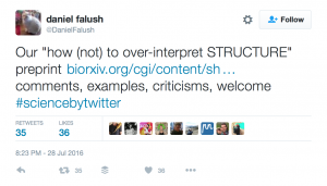
Several weeks ago1 Daniel Falush (@DanielFalush) posted a preprint on bioRxiv, “A tutorial on how (not) to over-interpret STRUCTURE/ADMIXTURE bar plots”. I finally had a chance to read it this weekend. Here’s the abstract:

Genetic clustering algorithms, implemented in popular programs such as STRUCTURE and ADMIXTURE, have been used extensively in the characterisation of individuals and populations based on genetic data. A successful example is reconstruction of the genetic history of African Americans who are a product of recent admixture between highly differentiated populations. Histories can also be reconstructed using the same procedure for groups which do not have admixture in their recent history, where recent genetic drift is strong or that deviate in other ways from the underlying inference model. Unfortunately, such histories can be misleading. We have implemented an approach (available at www.paintmychromsomes.com) to assessing the goodness of fit of the model using the ancestry ‘palettes’ estimated by CHROMOPAINTER and apply it to both simulated and real examples. Combining these complementary analyses with additional methods that are designed to test specific hypothesis allows a richer and more robust analysis of recent demographic history based on genetic data.

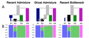
A key observation Falush and his co-authors make is that different demographic scenarios can lead to the same STRUCTURE diagram. They illustrate three different scenarios. In all of them, they simulate data from 12 populations but sample from only four of them. In all of the scenarios, population P4 has been isolated from the other three populations in the sample for a long time. It’s the relationship between P1, P2, and P3 that differs among the scenarios.

  • Recent admixture: P1 and P3 have also been distinct for some time, and P2 is a recent admixture of P1, P3, and P4.
  • Ghost admixture: P1 and P3 diverged some time ago, and P2 is a recent admixture of P1 and a “ghost” population more closely related to P3 than to P1.
  • Recent bottleneck: P1 is sister to P2 but underwent a strong recent bottleneck.

Screen Shot 2016-08-21 at 4.19.59 PM

As you can see, the STRUCTURE diagrams estimated from data simulated in each scenario are indistinguishable. They also show that if you have additional data available, specifically if you are lucky enough to be working in an organism with a lot of SNPs that are mapped, then you can combine estimates from CHROMOPAINTER with those from STRUCTURE to distinguish the recent admixture scenario from the other two – assuming that you’ve picked a reasonable number for K, the number of subpopulations.2

The authors also refer to Puechmaille’s recent work demonstrating that estimates of genetic structure are greatly affected by sample size. Bottom line: Read both this paper and Puechmaille’s if you use STRUCTURE, tread cautiously when interpreting results, and don’t expend too much effort trying to estimate the “right” K.


1OK, as you can see from the tweet, it was almost a month ago.

2The paper contains a brief remark about how hard it is to estimate K: “Unless the demographic history of the sample is particularly simple, the value of K inferred according to any statistically sensible criterion is likely to be smaller than the number of distinct drift events that have significantly impacted the sample. What the algorithm often does is in practice use variation in admixture proportions between individuals to approximately mimic the effect of more than K distinct drift events without estimating ancestral populations corresponding to each one.”

Falush, D., L. van Dorp, D. Lawson. 2016. A tutorial on how (not) to over-interpret STRUCTURE/ADMIXTURE bar plots. bioRxiv doi: 10.1101/066431
Lawson, D.J., G. Hellenthal, S. Myers, and D. Falush. 2012. Inference of population structure using dense haplotype data. PLoS Genetics 8:e1002453. doi: 10.1371/journal.pgen.1002453
Puechmaille, S.J. 2016. The program structure does not reliably recover the correct population structure when sampling is uneven: subsampling and new estimators alleviate the problem. Molecular Ecology Resources 16:608-627. doi: 10.1111/1755-0998.12512