Statistics

I’ve pointed out the problems with small, noisy samples using simulations (here, here, here, and here). But I’ve also learned that stories are far more persuasive than facts, and I’ve learned that I’m not good at telling stories. Fortunately, there are some people who tell stories very well, and John Schmidt is one of them. Here’s how his recent story, Noise Miners, starts.

What most people don’t understand about noise is how hard it is to find the good stuff.

You can get noise anywhere; most noise is just sitting on the ground, waiting for you to pick it up. Coincidences — “coinkidinks”, as collectors sometimes call them — can be had by the dozen just outside your front door. As I arrived in this small university town, home to one of the largest noise mines in the country, I planned to see how the high-quality noise was dug, and to learn about the often-forgotten people who dig it for us.

Follow the link and read the whole thing if that piques your interest.

I first mentioned the problems associated with small samples and noisy data in late August. That post demonstrated that you’d get the sign wrong almost half of the time with a small sample, even though a t-test would tell you that the result is statistically significant. The next two posts on the topic (September 9th and 19th) pointed out that being Bayesian won’t save you, even if you use fairly informative priors.

It turns out that I’m not alone in pointing out these problems. Caroline Tucker discusses a new paper in Ecology by Nathan Lemoine and colleagues that points out the same difficulties. She sums the problem up nicely.

It’s a catch-22 for small effect sizes: if your result is correct, it very well may not be significant; if you have a significant result, you may be overestimating the effect size.

There is no easy solution. Lemoine and his colleagues focus on errors of magnitude, where I’ve been focusing on errors in sign, but the bottom line is the same:

Be wary of results from studies with small sample sizes, even if the effects are statistically significant.

Lemoine, N.P., A. Hoffman, A.J. Felton, L. Baur, F. Chaves, J. Gray, Q. Yu, and M.D. Smith. 2016. Underappreciated problems of low replication in ecological field studies. Ecology doi: 10.1002/ecy.1506

Two weeks ago I pointed out that you should

Be wary of results from studies with small sample sizes, even if the effects are statistically significant.

Last week I pointed out that being Bayesian won’t save you. If you were paying close attention, you may have thought to yourself

Holsinger’s characterization of Bayesian inference isn’t completely fair. The mean effect sizes he simulated were only 0.05, 0.10, and 0.20, but he used a prior with a standard deviation of 1.0 in his analyses. Any Bayesian in her right mind wouldn’t use a prior that broad, because she’d have a clue going into the experiment that the effect size was relatively small. She’d pick a prior that more accurately reflects prior knowledge of the likely results.

It’s a fair criticism, so to see how much difference more informative priors make, I re-did the simulations with a Gaussian prior on each mean with a prior mean of 0.0 (as before) and a standard deviation of 2 times the effect size used in the simulation. Here are the results:

With a more informative prior, you’re not likely to say that an effect is positive when it’s actually negative. There are, however, a couple of things worth noticing when you compare this table to the last one.

1. The more informative prior doesn’t help much, if at all, with a sample size of 10. The N(0,1) prior got the sign wrong in 7 out of 62 cases where the 95% credible interval on the posterior mean difference did not include 0. The N(0,0.4) prior made the same mistake in 2 out of 22 cases. So it didn’t make as many mistakes as the less informative prior, but it made almost the same proportion. In other words, you’d be almost as likely to make a sign error with the more informative prior as you are with the less informative prior.
2. Even with a sample size of 100, you wouldn’t be “confident” that there is a difference very often (only 7 times out of 1000) when the “true” difference is small, 0.05, but you’d make a sign error nearly a third of the time (2 out of 7 cases) .

So what does all of this mean? When designing and interpreting an experiment you need to have some idea of how big the between-group differences you might reasonably expect to see are relative to the within-group variation. If the between-group differences are “small”, you’re going to need a “large” sample size to be confident about your inferences. If you haven’t collected your data yet, the message is to plan for “large” samples within each group. If you have collected your data and your sample size is small, be very careful about interpreting the sign of any observed differences – even if they are “statistically significant.”

What’s a “small” difference, and what’s a “large” sample? You can play with the R/Stan code in Github to explore the effects: https://github.com/kholsinger/noisy-data. You can also read Gelman and Carlin (Perspectives on Psychological Science 9:641; 2014 http://dx.doi.org/10.1177/1745691614551642) for more rigorous advice.

Last week I pointed out that you should

Be wary of results from studies with small sample sizes, even if the effects are statistically significant.

Now you may be thinking to yourself: “I’m a Bayesian, and I use somewhat informative priors. This doesn’t apply to me.” Well, I’m afraid you’re wrong. Here are results from analysis of data simulated according to the same conditions I used last week in exploring P-values. The prior on each mean is N(0, 1), and the prior on each standard deviation is half-N(0, 1).

Here “Power” refers to the number of times (out of 1000 replicates) the symmetric 95% credible intervals do not overlap 0, which is when we’d normally conclude we have evidence that the means of the two populations are different. Notice that when the effect and sample size are small (0.05 and 10, respectively), we would infer the wrong sign for the difference almost half of the time (18/39). We’re less likely to make a sign error when the effect is larger (7/62 for an effect of 0.20) or when the sample size is large (5/47 for a sample size of 100). But the bottom line remains the same:

Be wary of results from studies with small sample sizes, even if the effects are statistically significant.

This figure summarizes results from the simulation, and you’ll find the code in the same Github repository as the P-value code I mentioned last week: https://github.com/kholsinger/noisy-data. Remember that Gelman and Carlin (Perspectives on Psychological Science 9:641; 2014 http://dx.doi.org/10.1177/1745691614551642)  also have advice on how to tell whether you’re data are too noisy for your sample to give confidence in your inferences.

From a blog post Andrew Gelman made over a decade ago that I first came across about five or six years ago (http://andrewgelman.com/2004/12/29/type_1_type_2_t/):

In statistics, we learn about Type 1 and Type 2 errors. For example, from an intro stat book:

• A Type 1 error is committed if we reject the null hypothesis when it is true.
• A Type 2 error is committed if we accept the null hypothesis when it is false.

That’s a standard definition that anyone who’s had a basic statistics course has probably heard (even if they’ve forgotten it by now). Gelman points out, however, that it is arguably more useful to think about two different kinds of error,

• Type S errors occur when you claim that an effect is positive even though it’s actually negative.
• Type M errors occur when you claim that an effect is large when it’s really small (or vice versa).

You’re probably thinking to yourself, “Why should I care about Type S or Type M errors? Surely if I do a typical null hypothesis test and reject the null hypothesis, I won’t make a Type S error, right?”¹ Wrong! More precisely, you’re wrong if your sample size is small, and your data are noisy.

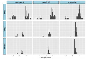
Let me illustrate this with a really simple example. Suppose we’re comparing the mean of two different populations x and y. To make that comparison, we take a sample of size N from each population, and perform a t-test (assuming equal variances in x and y). To make this concrete let’s assume that the variance is 1 in both populations and that the mean in population y is 0.05 greater than the mean in population x and suppose that N = 10. Now you’re probably thinking that the chances of detecting a difference between x and y isn’t great, and you’d be right. In fact, in the simulation below only 50 out of 1000 had a P-value < 0.05. What may surprise you is that of those 50 samples with P < 0.05, the mean of the sample from x was smaller than the mean of the sample from y. In other words, more than 30% of the time we would have made the wrong conclusion about which population had the larger mean, even though the difference in our sample was statistically significant. With a sample size of 100, we don’t pick up a significant difference between x and y that much more often (66 out of 1000 instead of 50 out of 1000), but only 9 of the 66 samples has the wrong sign. Obviously, if the difference in means is greater, sample size is less of an issue, but the bottom line is this:

If you are studying effects where between group differences are small relative to within group variation, you need a large sample to be confident in the sign of any effect you detect, even if the effect is statistically significant.

The figure below illustrates results for 1000 replicates drawn from two different populations with the specified difference in means and sample sizes. Source code (in R) to replicate the results and explore different combinations of sample size and mean difference is available in Github: https://github.com/kholsinger/noisy-data.

Gelman and Carlin (Perspectives on Psychological Science 9:641; 2014 http://dx.doi.org/10.1177/1745691614551642) provide a lot more detail and useful advice, including this telling paragraph from the conclusions:

[W]e believe that too many small studies are done and preferentially published when “significant.” There is a common misconception that if you happen to obtain statistical significance with low power, then you have achieved a particularly impressive feat, obtaining scientific success under difficult conditions.

Bottom line: Be wary of results from studies with small sample sizes, even if the effects are statistically significant.

¹I’m not going to talk about Type M errors, because in my work I’m usually happy just determining whether or not a given effect is positive and less worried about whether it’s big or small. If you’re worried about Type M errors, read the paper by Gelman and Tuerlinckx (PDF).