Statistics

I am about to begin developing a moderately complex mixed model in Stan to analyze realtinoships among anatomical/morphological traits (e.g., leaf thickness, LMA, wood density), physiological performance (e.g., A_max, stem hydraulic conductance), and indices of fitness (e.g., height, growth rate, number of seedheads). One complication is that the observations are from several different species of Protea at several different sites.¹ We’re going to treat sites as nested within species.

Before I start building the whole model, I wanted to make sure that I can do a simple mixed linear regression with a random site effect nested within a random species effect. In stan_lmer() notation that becomes:

stan_lmer(Amax ~ LMA + (1|Species/Site))

I ran a version of my code with several covariates in addition to LMA using hand-coded stan and compared the results to those from stan_lmer(). Estimates for the overall intercept and the regression coefficients associated with each covariate were very similar. The estimates of both standard deviations and individual random effects at the species and site within species level were rather different – especially at the species level. This was troubling, so I set up a simple simulation to see if I could figure out what was going on. The R code, Stan code, and simulation results are available in Github: https://kholsinger.github.io/mixed-models/.

The model used for simulation is very simple:

\(
\begin{equation}
y_k \sim \mbox{N}(\mu_k, \sigma) \\
\mu_k = \beta_0(species|site) + \beta_1x \\
\beta_0(species|site) \sim \mbox{N}(\beta_0(species), \sigma_{species|site}) \\
\beta_0(species) \sim \mbox{N}(\beta_0, \sigma_{species})
\end{equation}
\)

Happily, the Stan code I wrote does well in recovering the simulation parameters.² Surprisingly, it does better on recovering the random effect parameters than stan_lmer(). I haven’t completely sorted things out yet, but the difference is likely to be a result of different prior specifications for the random effects. My simulation code³ uses independent Cauchy(0,5) priors for the standard deviation of all variance parameters. stan_lmer() uses a covariance structure for all parameters that vary by group.⁴ If the difference in prior specifications is really responsible, it means that the differences between my approach and the approach used in stan_lmer() will vanish as the number of groups grows.

Since we’re only interested in the analog of \(\beta_1\) for the analyses we’ll be doing, the difference in random effect estimates doesn’t bother me, especially since my approach seems to recover them better given the random effect structure we’re working with. This is, however, a good reminder that if you’re working with mixed models and you’re interested in the group-level parameters, you’re going to need a large number of groups, not just a large number of individuals, to get reliable estimates of the group parameters.

(more…)

If you’ve spent any time using R, you probably know the name Hadley Wickham. He’s chief scientist at RStudio, the author of 4 books on R, and the author of several indispensable R packages, including ggplot2, dplyr, and devtools. I was reminded recently that several years ago, he wrote a very useful paper for the Journal of Statistical Software, “Tidy data” (August 2014, Volume 59, Issue 10, https://www.jstatsoft.org/article/view/v059i10).

If you are familiar with Hadley’s contributions to R, you won’t be surprised that tidy data has a simple, clean – tidy – set of requirements:

1. Each variable forms a column.
2. Each observation forms a row.
3. Each type of observational unit forms a table.

That sounds simple, but it requires that many of us rethink the way we structure our data, no more column headers as values, no more storing of multiple variables in one column, no more storing some variables in rows and others in columns. Fortunately, Hadley is also the author of tidyr. I haven’t used it yet, but given how bad I am at starting with tidy data, I suspect I’ll be using it a lot in the future.

Recently, a group of distinguished psychologists posted a preprint on PsyArxiv arguing for a re-definition of the traditional signifance threshold, lowering it from P < 0.05 to P < 0.005. They are concerned about reproducibility, and they argue that “changing the P value threshold is simple, aligns with the training undertaken by many researchers, and might quickly achieve broad acceptance.” That’s all true, but I’m afraid it won’t necessarily “improve the reproducibility of scientific research in many fields.”

Why? Let’s take a little trip down memory lane.

Almost a year ago I pointed out that we need to “Be wary of results from studies with small sample sizes, even if the effects are statistically significant.” I illustrated why with the following figure produced using R code available at Github: https://github.com/kholsinger/noisy-data

What that figure shows is the distribution of P-values that pass the P < 0.05 significance threshold when the true difference between two populations is mu standard deviations (with the same standard deviation in both populations) and with equal sample sizes of n. The results are from 1000 random replications. As you can see when the sample size is small, there’s a good chance that a significant result will have the wrong sign, i.e., the observed difference will be negative rather than positive, even if the between-population diffference is 0.2 standard deviations. When the between-population difference is 0.05, you’re almost as likely to say the difference is in the wrong direction as to get it right.

Does changing the threshold to P < 0.005 help. Well, I changed the number of replications to 10,000, reduced the threshold to P < 0.005, and here’s what I got.

Do you see a difference? I don’t. I haven’t run a formal statistical test to compare the distributions, but I’m pretty sure they’d be indistinguishable.

In short, reducing the significance threshold to P < 0.005 will result in fewer investigators reporting statistically significant results. But unless the studies they do also have reasonably large sample sizes relative to the expected magnitude of any effect and the amount of variability within classes, they won’t be any more likely to know the direction of the effect than with the traditional threshold of P < 0.05.

The solution to the reproducibility crisis is better data, not better statistics.

Lauren Kennedy and co-authors (citation below) worry about the effect of “contamination” on estimates of credible intervals.¹ The effect arises because we often assume that values are drawn from a normal distribution, even though there are “outliers” in the data, i.e., observations drawn from a different distribution that “contaminate” our observations. Not surprisingly, they find that a model including contamination does a “better job” of estimating the mean and credible intervals than one that assumes a simple normal distribution.²

They consider the following data as an example:
-2, -1, 0, 1, 2, 15
They used the following model for the data (writing in JAGS notation):

x[i] ~ dnorm(mu, tau)
tau ~ dgamma(0.0001, 0.0001)
mu ~ dnorm(0, 100)

That prior on tau should be a red flag. Gelman (citation below) pointed out a long time ago that such a prior is a long way from being vague or non-informative. It puts a tremendous amount of weight on very small values of tau, meaning a very high weight on large values of the variance. Similarly, the N(0, 100); prior on mu; may seem like a “vague” choice, but it puts more than 80% of the prior probability on outcomes with x < -20 or x > 20, substantially more extreme than any that were observed.

Before we begin an analysis we typically have some idea what “reasonable” values are for the variable we’re measuring. For example, if we are measuring the height of adult men, we would be very surprised to find anyone in our sample with a height greater than 3m or less than 0.5m. It wouldn’t make sense to use a prior for the mean that put appreciable probability on outcomes more extreme.

In this case the data are made up, so there isn’t any prior knowledge to work from. but the authors say that “[i]t is immediately obvious that the sixth data point is an outlier” (emphasis in the original). Let’s take them at their word. A reasonable choice of prior might then be N(0,1), since all of the values (except for the “outlier”) lie within two standard deviations of the mean.³ Similarly, a reasonable choice for the prior on sigma (sqrt(1/tau)) might be a half-normal with mean 0 and standard deviation 2, which will allow for standard deviations both smaller and larger than observed in the data.

I put that all together in a little R/Stan program (test.R, test.stan). When I run it, these are the results I get:

         mean se_mean    sd    2.5%     25%     50%     75%   97.5% n_eff  Rhat
mu      0.555   0.016 0.899  -1.250  -0.037   0.558   1.156   2.297  3281 0.999
sigma   4.775   0.014 0.841   3.410   4.156   4.715   5.279   6.618  3466 1.000
lp__  -16.609   0.021 0.970 -19.229 -17.013 -16.314 -15.903 -15.663  2086 1.001

Let’s compare those results to what Kennedy and colleagues report:

So if you use “reasonable” priors, you get a posterior mean from a model without contamination that isn’t very different from what you get from the more complicated contaminated normal model, and the credible intervals are actually narrower. If you really think a priori that 15 is an unreasonable observation, which estimate (point estimate and credible interval) would you prefer? I’d go for the model assuming a normal distribution with reasonable priors.

It all comes down to this. Your choice of priors matters. There is no such thing as an uninformative prior. If you think you are playing it safe by using very vague or flat priors, think carefully about what you’re doing. There’s a good chance that you’re actually putting a lot of prior weight on values that are unreasonable.⁴ You will almost always have some idea about what observations are reasonable or possible. Use that information to set weakly informative priors. See the discussion at https://github.com/stan-dev/stan/wiki/Prior-Choice-Recommendations for more detailed advice.

(more…)

Last week I pointed out a new paper by Denes Szucs and John Ioannidis, When null hypothesis significance testing is unsuitable for research: a reassessment.¹ I mentioned that P-values from small, noisy studies are likely to be misleading. Last April, Raghu Parthasarathy at The Eighteenth Elephant had a long post on a more fundamental problem with P-values: they encourage binary thinking. Why is this a problem?

1. “Binary statements can’t be sensibly combined” when measurements have noise.
2. “It is almost never necessary to combine boolean statements.”
3. “Everything always has an effect.”

Those brief statements probably won’t make any sense,² so head over to The Eighteenth Elephant to get the full explanation. The post is a bit long, but it’s easy to read, and well worth your time.

Andrew Gelman recently linked to Parthasarathy’s post and adds one more observation on how P-values are problematic: they are “interpretable only under the null hypothesis, yet the usual purpose of the p-value in practice is to reject the null.” In other words, P-values are derived assuming the null hypothesis is true. They tell us what the chances of getting the data we got are if the null hypothesis were true. Since we typically don’t believe the null hypothesis is true, the P-value doesn’t correspond to anything meaningful.

To take Gelman’s example, suppose we had an experiment with a control, treatment A, and treatment B. Our data suggest that treatment A is not different from control (P=0.13) but that treatment B is different from the control (P=0.003). That’s pretty clear evidence that treatment A and treatment B are different, right? Wrong.

P=0.13 corresponds to a treatment-control difference of 1.5 standard deviations; P=0.003, to a treatment-control difference of 3.0 standard deviations, a difference of 1.5 standard deviations, which corresponds to a P-value of 0.13. Why the apparent contradiction? Because if we want to say that treatment A and treatment B, we need to compare them directly to each other. When we do so, we realize that we don’t have any evidence that the treatments are different from one another.

As Parthasarthy points out in a similar example, a better interpretation is that we have evidence for the ordering (control < treatment A < treatment B). Null hypothesis significance testing could easily mislead us into thinking that what we have instead is (control = treatment A < treatment B). The problem arises, at least in part, because no matter how often we remind ourselves that it’s wrong to do so, we act as if a failure to reject the null hypothesis is evidence for the null hypothesis. Parthasarthy describes nicely how we should be approaching these problems:

It’s absurd to think that anything exists in isolation, or that any treatment really has “zero” effect, certainly not in the messy world of living things. Our task, always, is to quantify the size of an effect, or the value of a parameter, whether this is the resistivity of a metal or the toxicity of a drug.

We should be focusing on estimating the magnitude of effects and the uncertainty associated with those estimates, not testing null hypotheses.

(more…)

Several months ago I pointed out that P-values from small, noisy experiments are likely to be misleading. Given our training, we think that if a result is significant with a small sample, it must be a really big effect. But unless we have good reason to believe that there is very little noise in the results (a reason other than the small amount of variation observed in our sample), we could easily be misled. Not only will we overestimate how big the effect is, but we are almost as likely to say that the effect is positive when it’s really negative as we are to get the sign right. Look back at this post from August to see for yourself (and download the R code if you want to explore further). As Gelman and Carlin point out,

There is a common misconception that if you happen to obtain statistical significance with low power, then you have achieved a particularly impressive feat, obtaining scientific success under difficult conditions.

I bring this all up again because I recently learned of a new paper by Denes Szucs and John Ioannidis, When null hypothesis significance testing is unsuitable for research: a reassessment. They summarize their advice on null hypothesis significance testing (NHST) in the abstract:

Whenever researchers use NHST they should justify its use, and publish pre-study power calculations and effect sizes, including negative findings. Studies should optimally be pre-registered and raw data published.

They go on to point out that part of the problem is the way that scientists are trained:

(more…)

Remember Gelman’s preliminary principles for designing exploratory studies:

1. Validity and reliability of measurements.
2. Measuring lots of different things.
3. Connections between quantitative and qualitative data.
4. Collect or construct continuous measurements where possible.

I already wrote about validity and reliability. I admitted to not knowing enough yet to provide advice on assessing the reliability of measurements ecologists and evolutionists make (except in the very limited sense of whether or not repeated measurements of the same characteristic give similar results). For the time being that means I’ll focus on

• Remembering that I’m measuring an indicator of something else that is the thing that really matters, not the thing that really matters itself.
• Being as sure as I can that what I’m measuring is a valid and reliable indicator of that thing, even though the best I can do with that right now is a sort of heuristic connection between a vague notion of what I really think matters, underlying theory, and expectations derived from earlier work.

It’s that second part where “measuring lots of different things” comes in. Let’s go back to LMA and MAP. I’m interested in LMA because it’s an important component of the leaf economics spectrum. There are reasons to expect that tough leaves (those in which LMA is high) will not only be more resistant to herbivory from generalist herbivores, but that they will have lower rates of photosynthesis. Plants are investing more in those leaves. So high LMA is, in some vague sense, an indicator of the extent to which resource conservation is more important to plants than rapid acquisition of resources. So in designing an exploratory study, I should think about other traits plants have that could be indicators of resource conservation vs. rapid resource acquisition and measure as many of them as I can. A few that occur to me are leaf area, photosynthetic rate, leaf nitrogen content, leaf C/N ratio, tissue density, leaf longevity, and leaf thickness.

If I measure all of these (or at least several of them) and think of them as indicators of variation on the underlying “thing I really care about”, I can then imagine treating that underlying “thing I really care about” as a latent variable. One way, but almost certainly not the only way, I could assess the relationship between that latent variable and MAP would be to perform a factor analysis on the trait dataset, identify a single latent factor, and use that factor as the dependent variable whose variation I study in relation to MAP. Of course, MAP is only one way in which we might assess water availability in the environment. Others that might be especially relevant for perennials with long-lived leaves (like Protea) in the Cape Floristic Region rainfall seasonality, maximum number of days between days with “significant” rainfall in the summer, total summer rainfall, estimated potential evapotranspiration for the year, and estimated PET for the summer. A standard way to relate the “resource conservation” factor to the “water availability” factor would be a canonical correspondence analysis.

I am not advocating that we all start doing canonical correspondence analyses as our method of choice in designing exploratory studies, this way of thinking about exploratory studies does help me clarify (a bit) what it is that I’m really looking for. I still have work to do on getting it right, but it feels as if I’m heading towards something analogous to exploratory factor analysis (to identify factors that are valid, in the sense that they are interpretable and related in a meaningful way to existing theoretical constructs and understanding) and confirmatory factor analysis (to confirm that the exploration has revealed factors that can be reliably measured).

Stay tuned. It is likely to be a while before I have more thoughts to share, but as they develop, they’ll appear here, and if you follow along, you’ll be the first to hear about them.

On Wednesday I argued that we need carefully done exploratory studies to discover phenomena as much as we need carefully done experimental studies to test explanations for the phenomena that have been discovered.¹ Andrew Gelman suggests four preliminary principles:

1. Validity and reliability of measurements.
2. Measuring lots of different things.
3. Connections between quantitative and qualitative data.²
4. Collect or construct continuous measurements where possible.

Today I’m going to focus on #1, the validity and reliability of measurements.

If there happen to be any social scientists reading this, it’s likely to come as a shock to you to learn that most ecologists and evolutionary biologists haven’t thought too carefully about the problem of measurement, or at least that’s been my experience. My ecologist and evolutionary biologist friends are probably scratching their heads. “What the heck does Holsinger mean by ‘the problem of measurement.'” I’m sure I’m going to butcher this, because what little I think I know I picked up informally second hand, but here’s how I understand it.

(more…)

Andrew Gelman has a long, interesting, and important post about designing exploratory studies. It was inspired by the following comment from Ed Hagen following a blog post about a paper in Psychological Science.

Exploratory studies need to become a “thing”. Right now, they play almost no formal role in social science, yet they are essential to good social science. That means we need to put as much effort in developing standards, procedures, and techniques for exploratory studies as we have for confirmatory studies. And we need academic norms that reward good exploratory studies so there is less incentive to disguise them as confirmatory.

I think Ed’s suggestion is too narrow. Exploratory studies are essential to good science, not just good social science. We often (or at least I often) have only a vague idea about how features I’m interested in relate to one another. Take leaf mass per area (LMA)

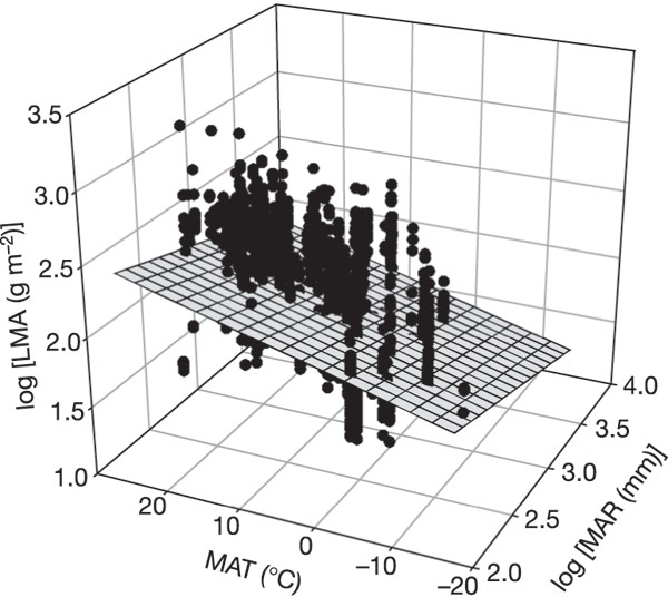
We often (or at least I often) have only a vague idea about how features I’m interested in relate to one another. Take leaf mass per area (LMA)¹ and mean annual temperature or mean annual precipitation, for example. In a worldwide dataset compiled by IJ Wright and colleagues², tougher leaves (higher values of LMA) are associated with warmer temperatures and less rainfall.

LMA, mean annual temperature, and log(mean annual rainfall) in 2370 species at 163 sites (from Wright et al. 2004)

We expected similar relationships in our analysis of Protea and Pelargonium,³ but we weren’t trying to test those expectations. We were trying to determine what those relationships were. We were, in other words, exploring our data, and guess what we found. Tougher leaves are associated with less rainfall in both general and with warmer temperatures in Protea. They were, however, associated with cooler temperatures in Pelargonium, exactly the opposite of what we expected. One reason for the difference might be that Pelargonium leaves are drought deciduous, so they avoid the summer drought characteristic of the regions from which our samples were collected. That is, of course, a post hoc explanation and has to be interpreted cautiously as a hypothesis to be tested, not as an established causal explanation. But that is precisely the point. We needed to investigate the phenomena to identify a pattern. Only then could we generate a hypothesis worth testing.

I find that I am usually more interested in discovering what the phenomena are than in tying down the mechanistic explanations for them. The problem, as Ed Hagen suggests, is that studies that explicitly label themselves as exploratory play little role in science. They tend to be seen as “fishing expeditions,” not serious science. The key, as Hagen suggests, is that to be useful, exploratory studies have to be done as carefully as explicit, hypothesis-testing confirmatory studies. A corollary he didn’t mention is that science will be well-served if we observe the distinction between exploratory and confirmatory studies.⁴

(more…)

Caroline Tucker reviewed a paper by Nathan Lemoine and colleagues in late September and reminded us that inferring anything from small, noisy samples is problematic.¹ Ramin Skibba now describes a good example of the problems that can arise.

In 1988, Fritz Strack and his colleagues reported that people found cartoons funnier if they held a pen in their teeth than if they held it between their lips. Why? Because holding a pen between your teeth causes you to smile, while holding one between your lips causes you to pout. This report spawned a series of studies on the “facial feedback hypothesis”, the hypothesis that facial expressions influence our emotional states. It seems plausible enough, and I know that I’ve read advice along this line in various places even though I’d never heard of the “facial feedback hypothesis” until I read Skibba’s article.

Unfortunately, the hypothesis wasn’t supported in what sounds like a pretty definitive study: 17 experiments and 1900 experimental subjects. Sixteen of the studies had large enough samples to be confident that the failure to detect an effect wasn’t a result of small sample size. Strack disagrees. He argues that (a) using a video camera to record participants may have made them self-conscious and suppressed their responses and (b) the cartoons were too old or too unfamiliar to participants to evoke an appropriate response.

Let’s take Strack at his word. Let’s assume he’s right on both counts. How important do you think the facial feedback to emotions is if being recorded by a video camera or being shown the wrong cartoons causes it to disappear (or at least to be undetectable)? I don’t doubt that Strack detected the effect in his sample, but the attempt to replicate his results suggest that the effect is either very sensitive to context or very weak.

I haven’t gone back to Strack’s paper to check on the original sample size, but the problem here is precisely what you’d expect to encounter if the original conclusions were based on a study in which the sample size was small relative to the signal-to-noise ratio. To reliably detect a small effect that varies across contexts requires either (a) very large sample size (if you want your conclusions to apply to the entire population) or (b) very careful specification of the precise subpopulation to which your conclusions apply (and extreme caution in attempting to generalize beyond it).

(more…)