
As we’ve seen in our discussion of AMOVA, nucleotide sequence data seem to have the potential to help us make not only evolutionary inferences about the sequences, but also about the evolutionary history of the populations from which we’ve collected those sequences. In the mid-1990s Alan Templeton introduced nested clade analysis as a formal approach to using an estimate of phylogenetic relationships among haplotypes to infer something both about the biogeographic history of the populations in which they are contained and the evolutionary processes associated with the pattern of diversification implied by the phylogenetic relationships among haplotypes and their geographic distribution. The statistical parsimony part of NCA depends heavily on coalescent theory for calculating the “limits” of parsimony. As a result, NCA combines aspects of pure phylogenetic inferenceparsimonywith aspects of pure population geneticscoalescent theoryto develop a set of inferences about the phylogeographic history of populations within species. So far as I am aware, no one uses NCA any more, but it is important to mention it as an early attempt to formalize the process of inferring the evolutionary history of populations from nucleotide sequence data. Prior to Templeton the process of inference was really just storytelling, storytelling that made a reasonablle amount of sense, but still storytelling. Now everyone uses methods based directly on coalescent theory or similar approaches. Before we get to that, though, I need to describe one complication that is taken for granted now that first became widely recognized in the late 1980s. Pekka Pamilo and Mashatoshi Nei pointed out that the phylogenetic relationships of a single gene might be different from those of the populations from which the samples were collected.
Gene trees describe the evolutionary relationships, i.e., the phylogeny of a set of genes. Population trees describe the phylogeny of a set of populations. We often want to infer the history of populations from a set of genes that we collect from those populations. There are several reasons why gene trees might not match population trees.
It could simply be a problem of estimation. Given a particular set of gene sequences, we estimate a phylogenetic relationship among them. But our estimate could be wrong. In fact, given the astronomical number of different trees possible with 50 or 60 distinct sequences, every phylogenetic estimate is virtually certain to be wrong somewhere. We just don’t know where. So a difference between our estimate of a gene tree and the population tree could mean nothing more than that they actually match, but our gene tree estimate is wrong.
There might have been a hybridization event in the past so that the phylogenetic history of the gene we’re studying is different from that of the populations from which we sampled. Hybridization is especially likely to have a large impact if the locus for which we have information is uniparentally inherited, e.g., mitochondrial or chloroplast DNA. A single hybridization event in the distant past in which the maternal parent was from a different population will give mtDNA or cpDNA a very different phylogeny than nuclear genes that underwent a lot of backcrossing after the hybridization event.
If the ancestral population was polymorphic at the time the initial split occurred alleles that are more distantly related might, by chance, end up in the same descendant population (see Figure 1)
As Pamilo and Nei showed, it’s possible to calculate the probability of discordance between the gene tree and the population tree using some basic ideas from coalescent theory. That leads to a further refinement, using coalescent theory directly to examine alternative biogeographic hypotheses.
Peter Beerli and Joe Felsenstein proposed a coalescent-based method to estimate migration rates among populations. As with other analytical methods we’ve encountered in this course, the details can get pretty hairy, but the basic idea is (relatively) simple.
Recall that in a single population we can describe the coalescent history of a sample without too much difficulty. Specifically, given a sample of \(k\) alleles in a diploid population with effective size \(N_e\), the probability that the first coalescent event took place \(t\) generations ago is \[P(t|k, N_e) = \left(\frac{k(k-1)}{4N_e}\right)\left(1- \frac{k(k-1)}{4N_e}\right)^{t-1} \quad . \label{eq:coalescent-single}\] Now suppose that we have a sample of alleles from \(K\) different populations. To keep things (relatively) simple, we’ll imagine that we have a sample of \(n\) alleles from every one of these populations and that every population has an effective size of \(N_e\). In addition, we’ll imagine that there is migration among populations, but again we’ll keep it really simple. Specifically, we’ll assume that the probability that a given allele in our sample from one population had its ancestor in a different population in the immediately preceding generation is \(m\).1 Under this simple scenario, we can again construct the coalescent history of our sample. How? Funny you should ask.
We start by using the same logic we used to construct equation ([eq:coalescent-single]). Specifically, we ask “What’s the probability of an ‘event’ in the immediately preceding generation?” The complication is that there are two kinds of events possible:
a coalescent event and
a migration event.
As in our original development of the coalescent process, we’ll assume that the population sizes are large enough that the probability of two coalescent events in a single time step is so small as to be negligible. In addition, we’ll assume that the number of populations and the migration rates are small enough that the probability of more than one event of either type is so small as to be negligible. That means that all we have to do is to calculate the probability of either a coalescent event or a migration event and combine them to calculate the probability of an event. It turns out that it’s easiest to calculate the probability that there isn’t an event first and then to calculate the probability that there is an event as one minus that.
We already know that the probability of a coalescent event in population \(k\), is \[P_k(\mbox{coalescent}|n, N_e) = \frac{k(k-1)}{4N_e} \quad ,\] so the probability that there is not a coalescent event in any of our \(K\) populations is \[P(\mbox{no coalescent}|k, N_e, K) = \left(1-\frac{k(k-1)}{4N_e}\right)^K \quad .\] If \(m\) is the probability that there was a migration event in a particular population than the probability that there is not a migration event involving any of our \(kK\) alleles2 is \[P(\mbox{no migration}|k,m, K) = (1-m)^{kK} \quad .\] So the probability that there is an event of some kind is \[P(\mbox{event}|k, m, N_e, K) = 1 - P(\mbox{no coalescent}|k, N_e, K)P(\mbox{no migration}|k,m, K) \quad .\label{eq:event}\] Now we can calculate the time back to the first event \[P(\mbox{event at }t|k, m, N_e, K) = P(\mbox{event}|k, m, N_e, K)\left(1 - P(\mbox{event}|k, m, N_e, K)\right)^{t-1} \quad . \label{eq:time-to-event}\] We can then use Bayes theorem to calculate the probability that the event was a coalescence or a migration and the population or populations involved. Notice, however, that if the event is a coalescent event, we first have to pick the population in which it occurred and then identify the pair of alleles that coalesced. Alleles have to be in the same population. Once we’ve done all of this, we have a new population configuration and we can start over. We continue until all of the alleles have coalesced into a single common ancestor, and then we have the complete coalescent history of our sample.3 That’s roughly the logic that Beerli and Felsenstein use to construct coalescent histories for a sample of alleles from a set of populationsexcept that they allow effective population sizes to differ among populations and they allow migration rates to differ among all pairs of populations. As if that weren’t bad enough, now things start to get even more complicated.
There are lots of different coalescent histories possible for a
sample consisting of \(n\) alleles from
each of \(K\) different populations,
even when we fix \(m\) and \(N_e\). Worse yet, given any one coalescent
history, there are a lot of different possible mutational histories
possible. In short, there are a lot of different possible sample
configurations consistent with a given set of migration rates and
effective population size. Nonetheless, some combinations of \(m\) and \(N_e\) will make the data more likely than
others. In other words, we can construct a likelihood for our data:
\[P(\mbox{data}|m, N_e) \propto f(n, m, N_e,
K) \quad ,\] where \(f(n, m,
N_e,K)\) is some very complicated function of the probabilities
we derived above. In fact, the function is so complicated, we can’t even
write it down. Fortunately, Beerli and Felsenstein, being very clever
people, figured out a way to simulate the likelihood, and
Migrate-n http://popgen.sc.fsu.edu/Migrate/Migrate-n.html provides
a (relatively) simple way that you can use your data to estimate \(m\) and \(N_e\) for a set of populations. In fact,
Migrate-N will allow you to estimate pairwise
migration rates among all populations in your sample, and since it can
simulate a likelihood, if you put priors on the parameters you’re
interested in, i.e., \(m\) and \(N_e\), you can get Bayesian estimates of
those parameters rather than maximum likelihood estimates, including
credible intervals around those estimates so that you have a good sense
of how reliable your estimates are.4
There’s one further complication I need to mention, and it involves a
lie I just told you. Migrate-N can’t give you
estimates of \(m\) and \(N_e\). Remember how every time we’ve dealt
with drift and another process we always end up with things like \(4N_em\), \(4N_e\mu\), and the like. Well, the
situation is no different here. What Migrate-N
can actually estimate are the two parameters \(4N_em\) and \(\theta=4N_e\mu\).5 How
did \(\mu\) get in here when I only
mentioned it in passing? Well, remember that I said that once the
computer has constructed a coalescent history, it has to apply mutations
to that history. Without mutation, all of the alleles in our sample
would be identical to one another. Mutation is what produces the
diversity. So what we get from Migrate-N isn’t
the fraction of a population that’s composed of migrants. Rather, we get
an estimate of how much migration contributes to local population
diversity relative to mutation. That’s a pretty interesting estimate to
have, but it may not be everything that we want.
There’s a further complication to be aware of. Think about the simulation process I described. All of the alleles in our sample are descended from a single common ancestor. That means we are implicitly assuming that the set of populations we’re studying have been around long enough and have been exchanging migrants with one another long enough that we’ve reached a drift-mutation-migration equilibrium. If we’re dealing with a relatively small number of populations in a geographically limited area, that may not be an unreasonable assumption, but what if we’re dealing with populations of crickets spread across all of the northern Rocky Mountains? And what if we haven’t sampled all of the populations that exist?6 In many circumstances, it may be more appropriate to imagine that populations diverged from one another at some time in the not too distant past, have exchanged genes since their divergence, but haven’t had time to reach a drift-mutation-migration equilibrium. What do we do then?
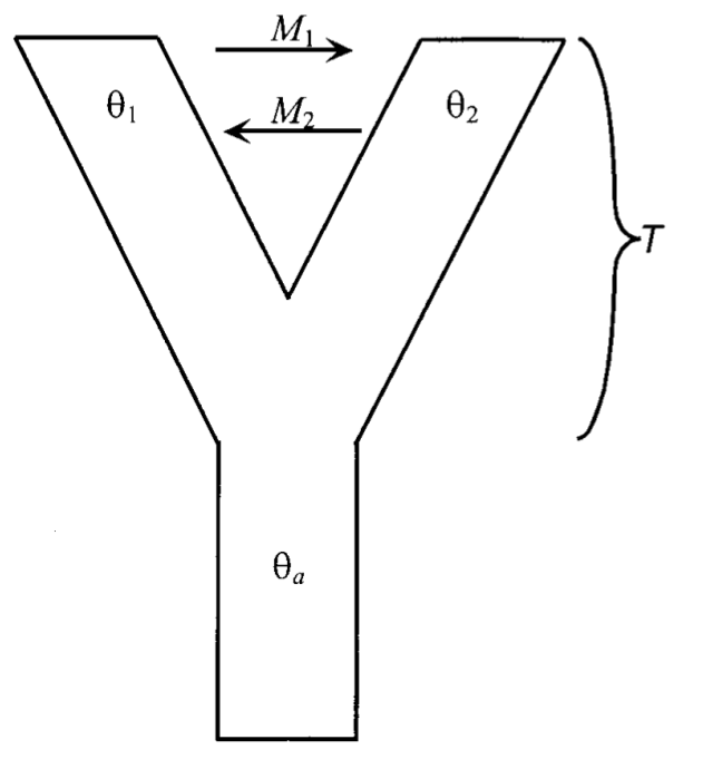
Rasmus Nielsen and John Wakely consider the simplest
generalization of Beerli and Felsenstein you
could imagine (Figure 2).
They consider a situation in which you have samples from only two
populations and you’re interested in determining both how long ago the
populations diverged from one another and how much gene exchange there
has been between the populations since they diverged. As in
Migrate-N mutation and migration rates are
confounded with effective population size, and the relevant parameters
become:
\(\theta_a\), which is \(4N_e\mu\) in the ancestral population.
\(\theta_1\), which is \(4N_e\mu\) in the first population.
\(\theta_2\), which is \(4N_e\mu\) in the second population.
\(M_1\), which is \(2N_em_1\) in the first population, where \(m_1\) is the fraction of the first population composed of migrants from the second population.
\(M_2\), which is \(2N_em_2\) in the second population.
\(T\), which is the time since the populations diverged. Specifically, if there have been \(t\) units since the two populations diverged, \(T=t/2N_1\), where \(N_1\) is the effective size of the first population.
Given that set of parameters, you can probably imagine that you can calculate the likelihood of the data for a given set of parameters.7 Once you can do that you can either obtain maximum-likelihood estimates of the parameters by maximizing the likelihood, or you can place prior distributions on the parameters and obtain Bayesian estimates from the posterior distribution. Either way, armed with estimates of \(\theta_a\), \(\theta_1\), \(\theta_2\), \(M_1\), \(M_2\), and \(T\) you can say something about:
the effective population sizes of the two populations relative to one another and relative to the ancestral population,
the relative frequency with which migrants enter each of the two populations from the other, and
the time at which the two populations diverged from one another.
Keep in mind, though, that the estimates of \(M_1\) and \(M_2\) confound local effective population sizes with migration rates. So if \(M_1 > M_2\), for example, it does not mean that the fraction of migrants incorporated into population 1 exceeds the fraction incorporated into population 2. It means that the number of migrants entering population 1 is greater than the number entering population 2.
Orti et al. report the results of phylogenetic analyses of mtDNA sequences from 25 populations of threespine stickleback, Gasterosteus aculeatus, in Europe, North America, and Japan. The data consist of sequences from a 747bp fragment of cytochrome \(b\). Nielsen and Wakely analyze these data using their approach. Their analyses show that “[a] model of moderate migration and very long divergence times is more compatible with the data than a model of short divergence times and low migration rates.” By “very long divergence times” they mean \(T > 4.5\), i.e., \(t > 4.5N_1\). Focusing on populations in the western (population 1) and eastern Pacific (population 2), they find that the maximum likelihood estimate of \(M_1\) is 0, indicating that there is little if any gene flow from the eastern Pacific (population 2) into the western Pacific (population 1). In contrast, the maximum likelihood estimate of \(M_2\) is about 0.5, indicating that one individual is incorporated into the eastern Pacific population from the western Pacific population every other generation. The maximum-likelihood estimates of \(\theta_1\) and \(\theta_2\) indicate that the effective size of the population eastern Pacific population is about 3.0 times greater than that of the western Pacific population.
Jody Hey later announced the release of
IMa2.8 Building on work
described in Hey and Nielsen ,
IMa2 allows you to estimate relative
divergence times, relative effective population sizes, and relative
pairwise migration rates for more than two populations at a time. That
flexibility comes at a cost, of course. In particular, you have to
specify the phylogenetic history of the populations before you begin the
analysis.
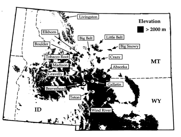
Lacey Knowles studied grasshoppers in the genus Melanopus. She collected 1275bp of DNA sequence data from cytochrome oxidase I (COI) from 124 individuals of M. oregonensis and two outgroup species. The specimens were collected from 15 “sky-island” sites in the northern Rocky Mountains (see Figure 3; ). Two alternative hypotheses had been proposed to describe the evolutionary relationships among these grasshoppers (refer to Figure 4 for a pictorial representation):
Widespread ancestor: The existing populations might represent independently derived remnants of a single, widespread population. In this case all of the populations would be equally related to one another.
Multiple glacial refugia: Populations that shared the same refugium will be closely related while those that were in different refugia will be distantly related.
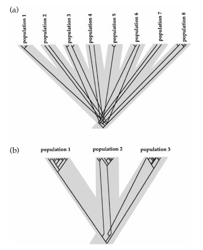
As is evident from Figure 4, the two hypotheses have very different consequences for the coalescent history of alleles in the sample. Since the interrelationships between divergence times and time to common ancestry differ so markedly between the two scenarios, the pattern of sequence differences found in relation to the geographic distribution will differ greatly between the two scenarios.
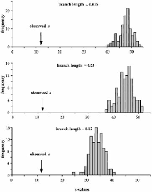
Using techniques described in Knowles and Maddison , Knowles simulated gene trees under the widespread ancestor hypothesis. She then placed them within a population tree representing the multiple glacial refugia hypothesis and calculated a statistic, \(s\), that measures the discordance between a gene tree and the population tree that contains it. This gave her a distribution of \(s\) under the widespread ancestor hypothesis. She compared the \(s\) estimated from her actual data with this distribution and found that the observed value of \(s\) was only 1/2 to 1/3 the size of the value observed in her simulations.9 Let’s unpack that a bit.
Knowles estimated the phylogeny of the haplotypes in her sample. \(s\) is the estimated minimum number of among-population migration events necessary to account for where haplotypes are currently found given the inferred phylogeny . Let’s call the \(s\) estimated from the data \(s_{obs}\).
Then she simulated a neutral coalescence process in which the populations were derived from a single, widespread ancestral population. For each simulation she rearranged the data so that populations were grouped into separate refugia and estimated \(s_{sim}\) from the rearranged data, and she repeated this 100 times for several different times since population splitting.
The results are shown in Figure 5. As you can see, the observed \(s\) value is much smaller than any of those obtained from the coalescent simulations. That means that the observed data require far fewer among-population migration events to account for the observed geographic distribution of haplotypes than would be expected with independent origin of the populations from a single, widespread ancestor. In short, Knowles presented strong evidence that her data are not consistent with the widespread ancestor hypothesis.
Approximate Bayesian Computation (ABC for short), extends the basic
idea Knowles used to consider more complicated scenarios. The
IMa approach developed by Nielsen, Wakely,
and Hey is potentially very flexible and
very powerful .
It allows for non-equilibrium scenarios in which the populations from
which we sampled diverged from one another at different times, but
suppose that we think our populations have dramatically increased in
size over time (as in humans) or dramatically changed their distribution
(as with an invasive species). Is there a way to use genetic data to
gain some insight into those processes? Would I be asking that question
if the answer were “No”?
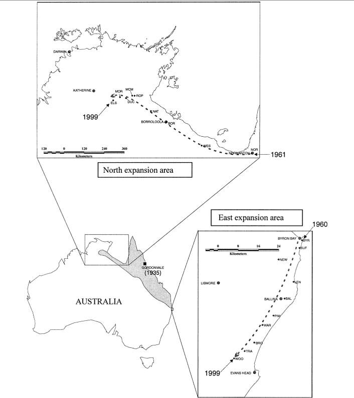
Let’s change things up a bit this time and start with an example of a problem we’d like to solve first. Once you see what the problem is, then we can talk about how we might go about solving it. The case we’ll discuss is the case of the cane toad, Bufo marinus, in Australia.
You may know that the cane toad is native to the American tropics. It was purposely introduced into Australia in 1935 as a biocontrol agent, where it has spread across an area of more than 1 million km\(^2\). Its range is still expanding in northern Australia and to a lesser extent in eastern Australia (Figure 6).10 Estoup et al. collected microsatellite data from 30 individuals in each of 19 populations along roughly linear transects in the northern and eastern expansion areas.
With these data they wanted to distinguish among five possible scenarios describing the geographic spread:
Isolation by distance: As the expansion proceeds, each new population is founded by or immigrated into by individuals with a probability proportional to the distance from existing populations.
Differential migration and founding: Identical to the preceding model except that the probability of founding a population may be different from the probability of immigration into an existing population.
“Island” migration and founding: New populations are established from existing populations without respect to the geographic distances involved, and migration occurs among populations without respect to the distances involved.
Stepwise migration and founding with founder events: Both migration and founding of populations occurs only among immediately adjacent populations. Moreover, when a new population is established, the number of individuals involved may be very small.
Stepwise migration and founding without founder events: Identical to the preceding model except that when a population is founded its size is assumed to be equal to the effective population size.
That’s a pretty complex set of scenarios. Clearly, you could use
Migrate or IMa2 to
estimate parameters from the data Estoup et al. report, but would those parameters
allow you to distinguish those scenarios? Not in any straightforward way
that I can see. Neither Migrate nor
IMa2 distinguishes between founding and
migration events for example. And with IMa2
we’d have to specify the relationships among our sampled populations
before we could make any of the calculations. In this case we want to
test alternative hypotheses of population relationship. So what do we
do?
Well, in principle we could take an approach similar to what
Migrate and IMa2
use. Let’s start by reviewing what we did last time11
with Migrate and
IMa2. In both cases, we knew how to simulate
data given a set of mutation rates, migration rates, local effective
population sizes, and times since divergence. Let’s call that whole,
long string of parameters \(\xi\) and
our big, complicated data set \(X\). If
we run enough simulations, we can keep track of how many of those
simulations produce data identical to the data we collected. With those
results in hand, we can estimate \(P(X|\xi)\), the likelihood of the data, as
the fraction of simulations that produce data identical to the data we
collected.12 In principle, we could take the
same approach in this, much more complicated, situation. But the problem
is that there are an astronomically large number of different possible
coalescent histories and different allelic configurations possible with
any one population history both because the population histories being
considered are pretty complicated and because the coalescent history of
every locus will be somewhat different from the coalescent history at
other loci. As a result, the chances of getting
any simulated samples that match our actual
samples is virtually nil, and we can’t estimate \(P(X|\xi)\) in the way we have so far.
Approximate Bayesian computation is an approach that allows us to get around this problem. It was introduced by Beaumont et al. precisely to allow investigators to get approximate estimates of parameters and data likelihoods in a Bayesian framework. Again, the details of the implementation get pretty hairy,13 but the basic idea is relatively straightforward.14
Calculate “appropriate” summary statistics for your data set, e.g., pairwise estimates of \(\phi_{ST}\) (possibly one for every locus if you’re using microsatellite or SNP data), estimates of within population diversity, counts of the number of segregating sites (for nucleotide sequence data, both within each population and across the entire sample) or counts of the number of segregating alleles (for microsatellite data). Call that set of summary statistics \(S\).
Specify a prior distribution for the unknown parameters, \(\xi\).
Pick a random set of parameter values, \(\xi'\) from the prior distribution and simulate a data set for that set of parameter values.
Calculate the same summary statistics for the simulated data set as you calculated for your actual data. Call that set of statistics \(S'\).
Calculate the distance between \(S\) and \(S'\).15 Call it \(\delta\). If it’s less than some value you’ve decided on, \(\delta^*\), keep track of \(S'\) and the associated \(\xi'\) and \(\delta\). Otherwise, throw all of them away and forget you ever saw them.
Return to step 2 and repeat until you have accepted a large number of pairs of \(S'\) and \(\xi'\).
Now you have a bunch of \(S'\)s and a bunch of \(\xi'\)s that produced them. Let’s label them \(S_i\) and \(\xi_i\), and let’s remember what we’re trying to do. We’re trying to estimate \(\xi\) for our real data. What we have from our real data is \(S\). So far it seems as if we’ve worked our computer pretty hard, but we haven’t made any progress.
Here’s where the trick comes in. Suppose we fit a regression to the data we’ve simulated \[\xi_i = \alpha + S_i\beta + \epsilon \quad ,\] where \(\alpha\) is an intercept, \(\beta\) is a vector of regression coefficients relating each of the summary statistics to \(\xi\), and \(\epsilon\) is an error vector.16 Once we’ve fit this regression, we can use it to predict what \(\xi\) should be in our real data, namely \[\xi = \alpha + S\beta \quad ,\] where the \(S\) here corresponds to our observed set of summary statistics. If we throw in some additional bells and whistles, we can approximate the posterior distribution of our parameters. With that we can get not only a point estimate for \(\xi\), but also credible intervals for all of its components.
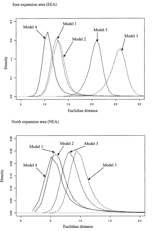
OK. So now we know how to do ABC, how do we apply it to the cane toad data. Well, using the additional bells and whistles I mentioned, we end up with a whole distribution of \(\delta\) for each of the scenarios we try. The scenario with the smallest \(\delta\) provides the best fit of the model to the data. In this case, that corresponds to model 4, the stepwise migration with founder model, although it is only marginally better than model 1 (isolation by distance) and model 2 (isolation by distance with differential migration and founding) in the northern expansion area (Figure 7).
Of course, we also have estimates for various parameters associated with this model:
\(N_{e_s}\): the effective population size when the population is stable.
\(N_{e_f}\): the effective population size when a new population is founded.
\(F_R\): the founding ratio, \(N_{e_s}/N_{e_f}\).
\(m\): the migration rate.
\(N_{e_s}m\): the effective number of migrants per generation.
The estimates are summarized in Table 1. Although the credible intervals are fairly broad,18 there are a few striking features that emerge from this analysis.
Populations in the northern expansion area are larger, than those in the eastern expansion region. Estoup et al. suggest that this is consistent with other evidence suggesting that ecological conditions are more homogeneous in space and more favorable to cane toads in the north than in the east.
A smaller number of individuals is responsible for founding new populations in the east than in the north, and the ratio of “equilibrium” effective size to the size of the founding population is bigger in the east than in the north. (The second assertion is only weakly supported by the results.)
Migration among populations is more limited in the east than in the north.
As Estoup et al. suggest, results like these could be used to motivate and calibrate models designed to predict the future course of the invasion, incorporating a balance between gene flow (which can reduce local adaptation), natural selection, drift, and colonization of new areas.
| Parameter | area | mean (5%, 90%) |
|---|---|---|
| \(N_{e_s}\) | east | 744 (205, 1442) |
| north | 1685 (526, 2838) | |
| \(N_{e_f}\) | east | 78 (48, 118) |
| north | 311 (182, 448) | |
| \(F_R\) | east | 10.7 (2.4, 23.8) |
| north | 5.9 (1.6, 11.8) | |
| \(m\) | east | 0.014 (\(6.0 \times 10^{-6}\), 0.064) |
| north | 0.117 (\(1.4 \times 10^{-4}\), 0.664) | |
| \(N_{e_s}m\) | east | 4.7 (0.005, 19.9) |
| north | 188 (0.023, 883) |
If you’ve learned anything by now, you should have learned that there
is no perfect method. An obvious disadvantage of ABC relative to either
Migrate or IMa2 is
that it is much more computationally intensive.
Because the scenarios that can be considered are much more complex, it simply takes a long time to simulate all of the data.
In the last few years, one of the other disadvantagesthat you had
to know how to do some moderately complicated scripting to piece
together several different packages in order to run analysishas become
less of a problem. popABC (http://code.google.com/p/popabc/,
DIYABC (http://www1.montpellier.inra.fr/CBGP/diyabc/), and the
abc library in R
make it relatively easy19
to perform the simulations.
Selecting an appropriate set of summary statistics isn’t easy, and it turns out that which set is most appropriate may depend on the value of the parameters that you’re trying to estimate and the which of the scenarios that you’re trying to compare is closest to the actual scenario applying to the populations from which you collected the data. Of course, if you knew what the parameter values were and which scenario was closest to the actual scenario, you wouldn’t need to do ABC in the first place.
In the end, ABC allows you to compare a small number of evolutionary scenarios. It can tell you which of the scenarios you’ve imagined provides the best combination of fit to the data and parsimonious use of parameters (if you choose model comparison statistics that include both components), but it takes additional work to determine whether the model is adequate, in the sense that it does a good job of explaining the data. Moreover, even if you determine that the model is adequate, you can’t exclude the possibility that there are other scenarios that might be equally adequateor even better.
These notes are licensed under the Creative Commons Attribution License. To view a copy of this license, visit or send a letter to Creative Commons, 559 Nathan Abbott Way, Stanford, California 94305, USA.