Introduction

So far in this course, we’ve focused on describing the pattern of variation within and among populations. We’ve talked about inbreeding, which causes genotype frequencies to change, although it leaves allele frequencies the same, and we’ve talked about how to describe variation among populations. But we haven’t yet discussed any evolutionary processes that could lead to a change in allele frequencies within populations.¹

Let’s return for a moment to the list of assumptions we developed when we derived the Hardy-Weinberg principle and see what we’ve done so far.

Assumption #1

Genotype frequencies are the same in males and females, e.g., $x_{11}$ is the frequency of the $A_1{A}_1$ genotype in both males and females.

Assumption #2

Genotypes mate at random with respect to their genotype at this particular locus.

Assumption #3

Meiosis is fair. More specifically, we assume that there is no segregation distortion, no gamete competition, no differences in the developmental ability of eggs, or the fertilization ability of sperm.

Assumption #4

There is no input of new genetic material, i.e., gametes are produced without mutation, and all offspring are produced from the union of gametes within this population.

Assumption #5

The population is of infinite size so that the actual frequency of matings is equal to their expected frequency and the actual frequency of offspring from each mating is equal to the Mendelian expectations.

Assumption #6

All matings produce the same number of offspring, on average.

Assumption #7

Generations do not overlap.

Assumption #8

There are no differences among genotypes in the probability of survival.

The only assumption we’ve violated so far is Assumption #2, the random-mating assumption. We’re going to spend the next several lectures talking about what happens when you violate Assumption #3, #6, or #8. When any one of those assumptions is violated we have some form of natural selection going on.²

Components of selection

Depending on which of those three assumptions is violated and how it’s violated we recognize that selection may happen in different ways and at different life-cycle stages.³

Assumption #3:

Meiosis is fair. There are at least two ways in which this assumption may be violated.

• Segregation distortion: The two alleles are not equally frequent in gametes produced by heterozygotes. The $t$-allele in house mice, for example, is found in 95% of fertile sperm produced by heterozygous males.

• Gamete competition: Gametes may be produced in equal frequency in heterozygotes, but there may be competition among them to produce fertilized zygotes, e.g., sperm competition in animals, pollen competition in seed plants.⁴

Assumption #6:

All matings produce the same number of progeny.

• Fertility selection: The number of offspring produced may depend on maternal genotype (fecundity selection), paternal genotype (virility selection), or on both.

Assumption #8:

Survival does not depend on genotype.

• Viability selection: The probability of survival from zygote to adult may depend on genotype, and it may differ between sexes.

At this point you’re probably thinking that I’ve covered all the possibilities. But by now you should also know me well enough to guess from the way I wrote that last sentence that if that’s what you were thinking, you’d be wrong. There’s one more way in which selection can happen that corresponds to violating

Asssumption #2:

Individuals mate at random.

• Sexual selection: Some individuals may be more successful at finding mates than others. Since females are typically the limiting sex (Bateman’s principle), the differences typically arise either as a result of male-male competition or female choice.

• Disassortative mating: When individuals preferentially choose mates different from themselves, rare genotypes are favored relative to common genotypes. This leads to a form a frequency-dependent selection.

The genetics of viability selection

That’s a pretty exhaustive (and exhausting) list of the ways in which selection can happen. We could spend the entire semester exploring each of those, but we’re going to focus in detail only on viability selection. Although I will say only a little about other forms of selection, it’s important to remember that any or all of the other forms of selection may be operating simultaneously on the genes or the traits that we’re studying, and the direction of selection due to these other components may be the same or different from the direction of viability selection. Remembering this is particularly important because there’s a tendency to think that viability selection is the only kind of natural selection there is.

We’re going to focus on viability selection for two reasons:

1. The most basic properties of natural selection acting on other components of the life history are similar to those of viability selection. A good understanding of viability selection provides a solid foundation for understanding other types of selection.⁵

2. The algebra associated with understanding viability selection is a lot simpler than the algebra associated with understanding any other type of selection, and the dynamics are simpler and easier to understand.⁶

The basic framework

To understand the basics, we’ll start with a numerical example using some data on Drosophila pseudoobscura that Theodosius Dobzhansky collected more than 70 years ago. You may remember that this species has chromosome inversion polymorphisms. Although these inversions involve many genes, they are inherited as if they were single Mendelian loci, so we can treat the karyotypes as single-locus genotypes and study their evolutionary dynamics. We’ll be considering two inversion types: the Standard inversion type, $ST$, and the Chiricahua inversion type, $CH$. We’ll use the following notation throughout our discussion:

The data look like this:⁷

Genotype and allele frequencies

It should be easy for you by this time to calculate the genotype frequencies in eggs and adults.⁸ I’ll refer to genotype frequencies in eggs (or newly-formed zygotes) as genotype frequencies before selection and genotype frequencies in adults as genotype frequencies after selection.

$$\begin{array}{rlr}\text{freq(}ST/ST\text{) before selection}& =& \frac{41}{41+82+27}\\ & =& 0.27\\ \text{freq(}ST/ST\text{) before selection}& =& \frac{N{x}_{11}}{N{x}_{11}+N{x}_{12}+N{x}_{22}}\\ & =& x_{11}\\ & & \\ \text{freq(}ST/ST\text{) after selection}& =& \frac{25}{25+74+12}\\ & =& 0.23\\ \text{freq(}ST/ST\text{) after selection}& =& \frac{w_{11}{x}_{11}N}{w_{11}{x}_{11}N+w_{12}{x}_{12}N+w_{22}{x}_{22}N}\\ & =& \frac{w_{11}{x}_{11}}{w_{11}{x}_{11}+w_{12}{x}_{12}+w_{22}{x}_{22}}\\ & =& \frac{w_{11}{x}_{11}}{\overline{w}}\\ \overline{w}& =& \frac{w_{11}{x}_{11}N+w_{12}{x}_{12}N+w_{22}{x}_{22}N}{N}\\ & =& w_{11}{x}_{11}+w_{12}{x}_{12}+w_{22}{x}_{22}.\end{array}$$ $\overline{w}$ is the mean fitness, i.e., the average probability of survival in the population.

If you followed that, you shouldn’t have much trouble following how to calculate the allele frequencies before and after selection:

$$\begin{array}{rlr}\text{freq(}ST\text{) before selection}& =& \frac{2(41)+82}{2(41+82+27)}\\ & =& 0.55\\ \text{freq(}ST\text{) before selection}& =& \frac{2(N{x}_{11})+N{x}_{12}}{2(N{x}_{11}+N{x}_{12}+N{x}_{22})}\\ & =& x_{11}+x_{12}/2\\ & & \\ \text{freq(}ST\text{) after selection}& =& \frac{2(25)+74}{2(25+74+12)}\\ & =& 0.56\\ \text{freq(}ST\text{) after selection}& =& \frac{2w_{11}{x}_{11}N+w_{12}{x}_{12}N}{2(w_{11}{x}_{11}N+w_{12}{x}_{12}N+w_{22}{x}_{22}N)}\\ & =& \frac{2w_{11}{x}_{11}+w_{12}{x}_{12}}{2(w_{11}{x}_{11}+w_{12}{x}_{12}+w_{22}{x}_{22})}\\ p^{\prime }& =& \frac{w_{11}{x}_{11}+w_{12}{x}_{12}/2}{w_{11}{x}_{11}+w_{12}{x}_{12}+w_{22}{x}_{22}}\\ x_{11}& =& p^2,x_{12}=2pq,x_{22}=q^2\\ p^{\prime }& =& \frac{w_{11}{p}^2+w_{12}pq}{w_{11}{p}^2+w_{12}2pq+w_{22}{q}^2}\\ \overline{w}& =& w_{11}{x}_{11}+w_{12}{x}_{12}+w_{22}{x}_{22}\\ & =& p^2{w}_{11}+2pq{w}_{12}+q^2{w}_{22}\end{array}$$

If you’re still awake, you’re probably wondering⁹ why I was able to substitute $p^2$, $2pq$, and $q^2$ for $x_{11}$, $x_{12}$, and $x_{22}$. Remember what I said earlier about what we’re doing here. The only Hardy-Weinberg assumption we’re violating is the one saying that all genotypes are equally likely to survive from zygote to adult. Remember also that a single generation in which all of the conditions for Hardy-Weinberg is enough to establish the Hardy-Weinberg proportions. Putting those two observations together, it’s not too hard to see that genotypes will be in Hardy-Weinberg proportions in newly formed zygotes. Viability selection will change the genotype frequencies later in the life-cycle, but we restart every generation with zygotes in the familiar Hardy-Weinberg proportions, $p^2$, $2pq$, and $q^2$, where $p$ is the frequency of $ST$ in the parents of those zygotes. An important implication of this that we’ll return to later, is that we can understand the dynamics of viability selection by focusing on how allele frequencies change. One of the reasons that other forms of natural selection are more complicated to understand is that we have to understand the dynamics of genotype frequencies, meaning that instead of one (relatively) simple equation we have at least two.

Selection acts on relative viability

Let’s stare at the selection equation for awhile and see what it means. $$p^{\prime }=\frac{w_{11}{p}^2+w_{12}pq}{\overline{w}}.$$ Suppose that instead of the fitnesses being $w_{11}$, $w_{12}$, and $w_{22}$ they were 1, $w_{12}/w_{11}$, and $w_{22}/w_{11}$. We’d then have the following equation: $$p^{\prime }=\frac{p^2+(w_{12}/w_{11})pq}{(\overline{w}/w_{11})}.$$ If you stare at that a bit, you’ll realize that equation ([eq:relative]) is equivalent to equation ([eq:absolute]), i.e., the way in which allele frequencies change from one generation to the next is identical in the two cases.¹⁰ I won’t write out all of the equations, but all these sets of fitnesses are equivalent to one another:¹¹

These observations illustrate the following general principle:

The consequences of natural selection (in an infinite population) depend only on the relative magnitude of fitnesses, not on their absolute magnitude.

That means, for example, that in order to predict the outcome of viability selection, we don’t have to know the probability that each genotype will survive, i.e., their absolute viabilities. We only need to know the probability that each genotype will survive relative to the probability that other genotypes will survive, i.e., their relative viabilities. As we’ll see later, it’s sometimes easier to estimate the relative viabilities than to estimate absolute viabilities.¹²

Marginal fitnesses

In case you haven’t already noticed, there’s almost always more than one way to write an equation.¹³ They’re all mathematically equivalent, but they emphasize different things. In this case, it can be instructive to look at the difference in allele frequencies from one generation to the next, $\mathrm{\Delta }p$: $$\begin{array}{rlr}\mathrm{\Delta }p& =& p^{\prime }-p\\ & =& \frac{w_{11}{p}^2+w_{12}pq}{\overline{w}}-p\\ & =& \frac{w_{11}{p}^2+w_{12}pq-\overline{w}p}{\overline{w}}\\ & =& \frac{p(w_{11}p+w_{12}q-\overline{w})}{\overline{w}}\\ & =& \frac{p(w_1-\overline{w})}{\overline{w}},\end{array}$$ where $w_1$ is the marginal fitness of allele $A_1$. To explain why it’s called a marginal fitness, I’d have to teach you some probability theory that you probably don’t want to learn.¹⁴ Fortunately, all you really need to know is that it corresponds to the probability that a randomly chosen $A_1$ allele in a newly formed zygote will survive into a reproductive adult.

Why do we care? Because it provides some (relatively obvious) intuition on how allele frequencies will change from one generation to the next. If $w_1>\overline{w}$, i.e., if the chances of a zygote carrying an $A_1$ allele of surviving to make an adult are greater than the chances of a randomly chosen zygote, then $A_1$ will increase in frequency. If $w_1<\overline{w}$, $A_1$ will decrease in frequency. Only if $p=0$, $p=1$, or $w_1=\overline{w}$ will the allele frequency not change from one generation to the next.

Patterns of natural selection

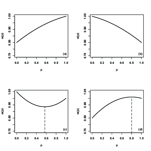
Well, all that algebra was lots of fun,¹⁵ but what good did it do us? Not an enormous amount, except that it shows us (not surprisingly), that allele frequencies are likely to change as a result of viability selection, and it gives us a nice little formula we could plug into a computer to figure out exactly how. One of the reasons that it’s useful¹⁶ to go through all of that algebra is that it allows us to make predictions about the consequences of natural selection simply by knowing the pattern of viability differences. What do I mean by pattern? Funny you should ask (Table 1).

Before exploring the consequences of these different patterns of natural selection, I need to introduce you to a very important result: Fisher’s Fundamental Theorem of Natural Selection. We’ll go through the details later when we get to quantitative genetics. In fact, we’ll derive Fisher’s Fundamental Theorem for one locus and two alleles. For now all you need to know is that viability selection causes the mean fitness of the progeny generation to be greater than or equal to the mean fitness of the parental generation, with equality only at equilibrium, i.e., $${\overline{w}}^{\prime }\ge \overline{w}.$$ How does this help us? Well, the best way to understand that is to illustrate how we can use Fisher’s theorem to predict the outcome of natural selection when we know only the pattern of viability differences. Let’s take each pattern in turn.

Directional selection

To use the Fundamental Theorem we plot $\overline{w}$ as a function of $p$ (Figure 1(a) and 1(b)). The Fundamental Theorem now tells us that allele frequencies have to change from one generation to the next in such a way that ${\overline{w}}^{\prime }>\overline{w}$, which can only happen if $p^{\prime }>p$. So viability selection will cause the frequency of the $A_1$ allele to increase in panel (a) and decrease in panel (b). Ultimately, the population will be monomorphic for the homozygous genotype with the highest fitness.¹⁷

Disruptive selection

If we plot $\overline{w}$ as a function of $p$ when $w_{11}>w_{12}$ and $w_{22}>w_{12}$, we see a very different pattern (Figure 1(c)). Since the Fundamental Theorem tells us that ${\overline{w}}^{\prime }\ge \overline{w}$, we know that if the population starts with an allele on the left side of the bowl $A_1$, will be lost. If it starts on the right side of the bowl, $A_2$ will be lost.¹⁸

Let’s explore this example a little further. To do so, I’m going to set $w_{11}=1+s_1$, $w_{12}=1$, and $w_{22}=1+s_2$.¹⁹ When fitnesses are written this way $s_1$ and $s_2$ are referred to as selection coefficients. Notice also with these definitions that the fitnesses of the homozygotes are greater than 1.²⁰ Using these definitions and plugging them into ([eq:absolute]), $$\begin{array}{rlr}{p}^{\prime }& =& \frac{p^2(1+s_1)+pq}{p^2(1+s_1)+2pq+q^2(1+s_2)}\\ & =& \frac{p(1+s_{1}p)}{1+p^2{s}_1+q^2{s}_2}.\end{array}$$ We can use equation ([eq:disruptive]) to find the equilibria of this system, i.e., the values of $p$ such that $p^{\prime }=p$. $$\begin{array}{rlr}p& =& \frac{p(1+s_{1}p)}{1+p^2{s}_1+q^2{s}_2}\\ p(1+p^2{s}_1+q^2{s}_2)& =& p(1+s_{1}p)\\ p((1+p^2{s}_1+q^2{s}_2)-(1+s_{1}p))& =& 0\\ p(p{s}_1(p-1)+q^2{s}_2)& =& 0\\ p(-pq{s}_1+q^2{s}_2)& =& 0\\ pq(-p{s}_q+q{s}_2)& =& 0.\end{array}$$ So the population is at equilibrium with $p^{\prime }=p$ if $\hat{p}=0$, $\hat{q}=0$, or $\hat{p}{s}_1=\hat{q}{s}_2$.²¹ We can simplify that last one a little further, too. $$\begin{array}{rlr}\hat{p}{s}_1& =& \hat{q}{s}_2\\ \hat{p}{s}_1& =& (1-\hat{p})s_2\\ \hat{p}(s_1+s_2)& =& s_2\\ \hat{p}& =& \frac{s_2}{s_1+s_2}.\end{array}$$

Fisher’s Fundamental Theorem tells us which of these equilibria matter. I’ve already mentioned that depending on which side of the bowl you start, you’ll either lose the $A_1$ allele or the $A_2$ allele. But suppose you happen to start exactly at the bottom of the bowl. That corresponds to the equilibrium with $\hat{p}=s_2/(s_1+s_2)$. What happens then?

Well, if you start exactly there, you’ll stay there forever (in an infinite population). But if you start ever so slightly off the equilibrium, you’ll move farther and farther away. It’s what mathematicians call an unstable equilibrium. Any departure from that equilibrium gets larger and larger. For evolutionary purposes, we don’t have to worry about a population getting to an unstable equilibrium. It never will. Unstable equilibria are ones that populations evolve away from.

When a population has only one allele present it is said to be fixed for that allele. Since having only one allele is also an equilibrium (in the absence of mutation), we can also call it a monomorphic equilibrium. When a population has more than one allele present, it is said to be polymorphic. If two or more alleles are present at an equilibrium, we can call it a polymorphic equilibrium. Thus, another way to describe the results of disruptive selection is to say that the monomorphic equilibria are stable, but that the polymorphic equilibrium is not.²²

Stabilizing selection

If we plot $\overline{w}$ as a function of $p$ when $w_{11}<w_{12}$ and $w_{22}<w_{12}$, we see a third pattern. The plot is shaped like an upside down bowl (Figure 1).

In this case we can see that no matter what allele frequency the population starts with, the only way that ${\overline{w}}^{\prime }\ge \overline{w}$ can hold is if the allele frequency changes in such a way that in every generation it gets closer to the value where $\overline{w}$ is maximized. Unlike directional selection or disruptive selection, in which natural selection tends to eliminate one allele or the other, stabilizing selection tends to keep both alleles in the population. You’ll also see this pattern of selection referred to as balancing selection, because the selection on each allele is “balanced” at the polymorphic equilibria.²³ We can summarize the results by saying that the monomorphic equilibria are unstable and that the polymorphic equilibrium is stable. By the way, if we write the fitness as $w_{11}=1-s_1$, $w_{12}=1$, and $w_{22}=1-s_2$, then the allele frequency at the polymorphic equilibrium is $\hat{p}=s_2/(s_1+s_2)$.²⁴ Notice that $\hat{p}$ depends only on the ratio of $s_1$ to $s_2$, not the magnitude. Again, it is only relative fitnesses that matter.

Fertility selection

So far we’ve been talking about natural selection that occurs as a result of differences in the probability of survival, i.e., viability selection. There are, of course, other ways in which natural selection can occur:

• Heterozygotes may produce gametes in unequal frequencies, segregation distortion, or gametes may differ in their ability to participate in fertilization, gametic selection.²⁵

• Some genotypes may be more successful in finding mates than others, sexual selection.

• The number of offspring produced by a mating may depend on maternal and paternal genotypes, fertility selection.

In fact, most studies that have measured components of selection have identified far larger differences due to fertility than to viability. Thus, fertility selection is a very important component of natural selection in most populations of plants and animals. As we’ll see a little later, it turns out that sexual selection is mathematically equivalent to a particular type of fertility selection. But before we get to that, let’s look carefully at the mechanics of fertility selection.

Formulation of fertility selection

It is useful to describe patterns of fertility selection in terms of a fitness matrix. Describing the matrix is easy. Writing it down gets messy. Each element in the table is simply the average number of offspring produced by a given mated pair. We write down the table with paternal genotypes in columns and maternal genotypes in rows:

Then the frequency of genotype $A_1{A}_1$ after one generation of fertility selection is:²⁶ $$x_{11}^{\prime }=\frac{x_{11}^2{F}_{11,11}+x_{11}{x}_{12}(F_{11,12}+F_{12,11})/2+(x_{12}^2/4)F_{12,12}}{\overline{F}},$$ where $\overline{F}$ is the mean fecundity of all matings in the population.²⁷

It probably won’t surprise you to learn that it’s very difficult to say anything very general about how genotype frequenices will change when there’s fertility selection. Not only are there nine different fitness parameters to worry about, but since genotypes are never guaranteed to be in Hardy-Weinberg proportion, all of the algebra has to be done on a system of three simultaneous equations.²⁸ There are three weird properties that I’ll mention:

1. ${\overline{F}}^{\prime }$ may be smaller than $\overline{F}$. Unlike selection on viabilities in which fitness evolved to the maximum possible value, there are situations in which fitness will evolve to the minimum possible value when there’s selection on fertilities.²⁹

2. A high fertility of heterozygote $\times$ heterozygote matings is not sufficient to guarantee that the population will remain polymorphic.

3. Selection may prevent loss of either allele, but there may be no stable equilibria.

Conditions for protected polymorphism

There is one case in which it’s fairly easy to understand the consequences of selection, and that’s when one of the two alleles is very rare. Suppose, for example, that $A_1$ is very rare, then a little algebraic trickery³⁰ shows that $$\begin{array}{rlr}{x}_{11}^{\prime }& \approx & 0\\ x_{12}^{\prime }& \approx & \frac{x_{12}(F_{12,22}+F_{22,12})/2}{F_{22,22}}\end{array}$$ So $A_1$ will become more frequent if $$(F_{12,22}+F_{22,12})/2>F_{22,22}$$ Similarly, $A_2$ will become more frequent when it’s very rare when $$(F_{11,12}+F_{12,11})/2>F_{11,11}.$$ If both equation ([eq:a-1]) and ([eq:a-2]) are satisfied, natural selection will tend to prevent either allele from being eliminated. We have what’s known as a protected polymorphism.

Conditions ([eq:a-1]) and ([eq:a-2]) are fairly easy to interpret intuitively: There is a protected polymorphism if the average fecundity of matings involving a heterozygote and the “resident” homozygote exceeds that of matings of the resident homozygote with itself.³¹

NOTE: It’s entirely possible for neither inequality to be satisfied and for their to be a stable polymorphism. In other words, depending on where a population starts, selection may eliminate one allele or the other or keep both segregating in the population in a stable polymorphism.³²

Creative Commons License

These notes are licensed under the Creative Commons Attribution License. To view a copy of this license, visit or send a letter to Creative Commons, 559 Nathan Abbott Way, Stanford, California 94305, USA.