Introduction to quantitative genetics

So far in this course we have dealt entirely either with the evolution of characters that are controlled by simple Mendelian inheritance at a single locus or with the evolution of molecular sequences. Even on Tuesday when we were dealing with population genomic data, data from hundreds or thousands of loci, we were treating the variation at each locus separately and combining results across loci. I have some old notes on gametic disequilibrium and how allele frequencies change at two loci simultaneously, but they’re in the “Old notes, no longer updated” section of the book version of these notes (https://figshare.com/articles/journal_contribution/Lecture_notes_in_population_genetics/100687), and we didn’t discuss them.1 In every example we’ve considered so far we’ve imagined that we could understand something about evolution by examining the evolution of a single gene. That’s the domain of classical population genetics.

For the next few weeks we’re going to be exploring a field that’s older than classical population genetics, although the approach we’ll be taking to it involves the use of population genetic machinery.2 If you know a little about the history of evolutionary biology, you may know that after the rediscovery of Mendel’s work in 1900 there was a heated debate between the “biometricians” (e.g., Galton and Pearson) and the “Mendelians” (e.g., de Vries, Correns, Bateson, and Morgan).

Biometricians asserted that the really important variation in evolution didn’t follow Mendelian rules. Height, weight, skin color, and similar traits seemed to

Since variation in such quantitative traits seemed to be more obviously related to organismal adaptation than the “trivial” traits that Mendelians studied, it seemed obvious to the biometricians that Mendelian geneticists were studying a phenomenon that wasn’t particularly interesting.

Mendelians dismissed the biometricians, at least in part, because they seemed not to recognize the distinction between genotype and phenotype. It seemed to at least some Mendelians that traits whose expression was influenced by the environment were, by definition, not inherited. Moreover, the evidence that Mendelian principles accounted for the inheritance of many discrete traits was incontrovertible.

Woltereck’s  experiments on Daphnia helped to show that traits whose expression is environmentally influenced may also be inherited. He introduced the idea of a norm of reaction to describe the observation that the same genotype may produce different phenotypes in different environments (Figure 1). When you fertilize a plant, for example, it will grow larger and more robust than when you don’t. The phenotype an organism expresses is, therefore, a product of both its genotype and its environment.

Hypothetical illustration of reaction norms for two genotypes across a 1-dimensional environmental gradient (from Wikipedia, Public Domain, 
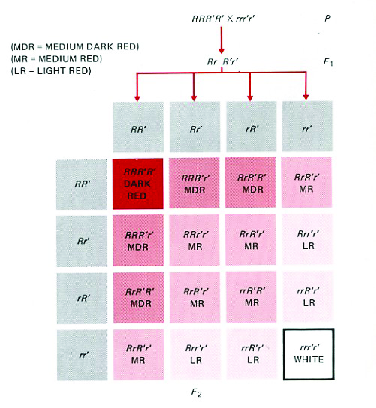
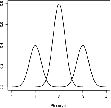
https://en.wikipedia.org/w/index.php?curid=3925138, accessed 9 April 2017).

Nilsson-Ehle’s  experiments on inheritance of kernel color in wheat showed how continuous variation and Mendelian inheritance could be reconciled (Figure 2). He demonstrated that what appeared to be continuous variation in color from red to white with blending inheritance could be understood as the result of three separate genes influencing kernel color that were inherited separately from one another. It was the first example of what’s come to be known as polygenic inheritance. Fisher , in a paper that grew out of his undergraduate Honors thesis at Cambridge University, set forth the mathematical theory that describes how it all works. That’s the theory of quantitative genetics, and it’s what we’re going to spend the rest of the course discussing.

Results from one of Nilsson-Ehle’s crosses illustrating polygenic inheritance of kernel color in wheat (from http://www.biology-pages.info/Q/QTL.html, accessed 9 April 2017).

An overview of where we’re headed

Woltereck’s ideas force us to realize that when we see a phenotypic difference between two individuals in a population there are three possible sources for that difference:

  1. The individuals have different genotypes.

  2. The individuals developed in different environments.

  3. The individuals have different genotypes and they developed in different environments.

This leads us naturally to think that phenotypic variation consists of two separable components, namely genotypic and environmental components.3 Putting that into an equation \[\mbox{Var}(P) = \mbox{Var}(G) + \mbox{Var}(E) \quad ,\] where \(\mbox{Var}(P)\) is the phenotypic variance, \(\mbox{Var}(G)\) is the genetic variance, and \(\mbox{Var}(E)\) is the environmental variance.4 As we’ll see in just a moment, we can also partition the genetic variance into components, the additive genetic variance, \(\mbox{Var}(A)\), and the dominance variance, \(\mbox{Var}(D)\).5

There’s a surprisingly subtle and important insight buried in that very simple equation: Because the expression of a quantitative trait is a result both of genes involved in that trait’s expression and the environment in which it is expressed, it doesn’t make sense to say of a particular individual’s phenotype that genes are more important than environment in determining it. You wouldn’t have a phenotype without both. At most what we can say is that when we look at a particular population of organisms in a particular environment, some fraction of the phenotypic variation they exhibit is due to differences in the genes they carry and that some fraction is due to differences in the environment they have experienced.6 If we have two individuals with different phenotypes, e.g., Ralph is tall and Harry is short, we can’t even say whether the difference between Ralph and Harry is because of differences in their genes or differences in their developmental environment.

One important implication of this insight is that much of the “nature vs. nurture” debate concerning human intelligence or human personality characteristics is misguided. The intelligence and personality that you have is a product of both the genes you happened to inherit and the environment that you happened to experience. Any differences between you and the person next to you probably reflect both differences in genes and differences in environment. Moreover, even if the differences between you and your neighbor are due to differences in genes, it doesn’t mean that those differences are fixed and indelible. You may be able to do something to change them.

Take phenylketonuria, for example. It’s a condition in which individuals are homozygous for a deficiency that prevents them from metabolizing phenylalanine (https://medlineplus.gov/phenylketonuria.html). If individuals with phenylketonuria eat a normal diet, severe intellectual disabilities can result by the time an infant is one year old. But if they eat a diet that is very low in phenylalanine, their development is completely normal. In other words, clear genetic differences at this locus can lead to dramatic differences in cognitive ability, but they don’t have to.

It’s often useful to talk about how much of the phenotypic variance is a result of additive genetic variance or of genetic variance. \[h^2_n = \frac{\mbox{Var}(A)}{\mbox{Var}(P)}\] is what’s known as the narrow-sense heritability. It’s the proportion of phenotypic variance that’s attributable to differences among individuals in their additive genotype,7 much as \(F_{st}\) can be thought of as the proportion of genotypic diversity that attributable to differences among populations. Similarly, \[h^2_b = \frac{\mbox{Var}(G)}{\mbox{Var}(P)}\] is the broad-sense heritability. It’s the proportion of phenotypic variance that’s attributable to differences among individuals in their genotype. It is not, repeat NOT, a measure of how important genes are in determining phenotype. Every individuals phenotype is determined both by its genes and by its phenotype. It measures how much of the difference among individuals is attributable to differences in their genes.8 Why bother to make the distinction between narrow- and broad-sense heritability? Because, as we’ll see, it’s only the additive genetic variance that responds to natural selection.9 In fact, \[R = h^2_nS \quad ,\] where \(R\) is the response to selection and \(S\) is the selective differential.

As you’ll see in the coming weeks, there’s a lot of stuff hidden behind these simple equations, including a lot of assumptions. But quantitative genetics is very useful. Its principles have been widely applied in plant and animal breeding for more than a century, and they have been increasingly applied in evolutionary investigations in the last forty years.10.

Partitioning the phenotypic variance

Before we worry about how to estimate any of those variance components I just mentioned, we first have to understand what they are. So let’s start with some definitions (Table 1).11

Fundamental parameter definitions for quantitative genetics with one locus and two alleles.
Genotype \(A_1A_1\) \(A_1A_2\) \(A_2A_2\)
Frequency \(p^2\) \(2pq\) \(q^2\)
Genotypic value \(x_{11}\) \(x_{12}\) \(x_{22}\)
Additive genotypic value \(2\alpha_1\) \(\alpha_1 + \alpha_2\) \(2\alpha_2\)

You should notice something rather strange about Table 1 when you look at it. I motivated the entire discussion of quantitative genetics by talking about the need to deal with variation at many loci, and what I’ve presented involves only two alleles at a single locus. I do this for two reasons:

  1. It’s not too difficult to do the algebra with multiple alleles at one locus instead of only two, but it gets messy, doesn’t add any insight, and I’d rather avoid the mess.

  2. Doing the algebra with multiple loci involves a lot of assumptions, which I’ll mention when we get to applications, and the algebra is even worse than with multiple alleles.

Fortunately, the basic principles extend with little modification to multiple loci, so we can see all of the underlying logic by focusing on one locus with two alleles where we have a chance of understanding what the different variance components mean.

Two terms in Table 1 will almost certainly be unfamiliar to you: genotypic value and additive genotypic value. Of the two, genotypic value is the easiest to understand (Figure 3). It simply refers to the average phenotype associated with a given genotype.12 The additive genotypic value refers to the average phenotype associated with a given genotype, as would be inferred from the additive effect of the alleles of which it is composed. That didn’t help much, did it? That’s because I now need to tell you what we mean by the additive effect of an allele.13

The phenotype distribution in a population in which the three genotypes at a single locus with two alleles occur in Hardy-Weinberg proportions and the alleles occur in equal frequency. The \(A_1A_1\) genotype has a mean trait value of 1, the \(A_1A_2\) genotype has a mean trait value of 2, and the \(A_2A_2\) genotype has a mean trait value of 3, but each genotype can produce a range of phenotypes with the standard deviation of the distribution being 0.25 in each case.

The additive effect of an allele

In constructing Table 1 I used the quantities \(\alpha_1\) and \(\alpha_2\), but I didn’t tell you where they came from. Obviously, the idea should be to pick values of \(\alpha_1\) and \(\alpha_2\) that give additive genotypic values that are reasonably close to the genotypic values. A good way to do that is to minimize the squared deviation between the two, weighted by the frequency of the genotypes. So our first big assumption is that genotypes are in Hardy-Weinberg proportions.14

The objective is to find values for \(\alpha_1\) and \(\alpha_2\) that minimize: \[a = p^2[x_{11}-2\alpha_1]^2 + 2pq[x_{12}-(\alpha_1+\alpha_2)]^2 + q^2[x_{22}-2\alpha_2]^2 \quad .\] To do this we take the partial derivative of \(a\) with respect to both \(\alpha_1\) and \(\alpha_2\), set the resulting pair of equations equal to zero, and solve for \(\alpha_1\) and \(\alpha_2\).15 \[\begin{aligned} \frac{\partial a}{\partial{\alpha_1}} &=& p^2\{2[x_{11} - 2\alpha_1][-2]\} + 2pq\{2[x_{12} - (\alpha_1+\alpha_2)][-1]\} \\ &=& -4p^2[x_{11} - 2\alpha_1] -4pq[x_{12} - (\alpha_1+\alpha_2)] \\ \frac{\partial a}{\partial{\alpha_2}} &=& q^2\{2[x_{22} - 2\alpha_2][-2]\} + 2pq\{2[x_{12} - (\alpha_1+\alpha_2)][-1]\} \\ &=& -4q^2[x_{22} - 2\alpha_2] -4pq[x_{12} - (\alpha_1+\alpha_2)] \end{aligned}\] Thus, \(\frac{\partial a}{\partial{\alpha_1}} = \frac{\partial a}{\partial{\alpha_2}} = 0\) if and only if \[\begin{aligned} p^2(x_{11} - 2\alpha_1) + pq(x_{12} - \alpha_1 - \alpha_2) &=& 0 \nonumber \\ q^2(x_{22} - 2\alpha_2) + pq(x_{12} - \alpha_1 - \alpha_2) &=& 0 \label{eq:zeros} \end{aligned}\] Adding the equations in ([eq:zeros]) we obtain (after a little bit of rearrangement) \[- [p^2(2\alpha_1) + 2pq(\alpha_1 + \alpha_2) + q^2(2\alpha_2)] = 0 \quad . \label{eq:basic}\]

Now the first term in square brackets is just the mean phenotype in the population, \(\bar x\). Thus, we can rewrite equation ([eq:basic]) as: \[\begin{aligned} {\bar x} &=& 2p^2\alpha_1 + 2pq(\alpha_1 + \alpha_2) +2q^2\alpha_2 \nonumber \\ &=& 2p\alpha_1(p+q) + 2q\alpha_2(p+q) \nonumber \\ &=& 2(p\alpha_1 + q\alpha_2) \quad . \label{eq:alpha_bar} \end{aligned}\] That hasn’t helped us figure out what \(\alpha_1\) and \(\alpha_2\) are, but it will turn out to be useful later, trust me.

Now divide the first equation in ([eq:zeros]) by \(p\) and the second by \(q\). \[\begin{aligned} p(x_{11} - 2\alpha_1) + q(x_{12} - \alpha_1 - \alpha_2) &=& 0 \label{eq:zeros_divide_1} \\ q(x_{22} - 2\alpha_2) + p(x_{12} - \alpha_1 - \alpha_2) &=& 0 \quad . \label{eq:zeros_divide_2} \end{aligned}\] Thus, \[\begin{aligned} px_{11} + qx_{12} &=& 2p\alpha_1 + q\alpha_1 + q\alpha_2 \\ &=& \alpha_1(p + q) + p\alpha_1 + q\alpha_2 \\ &=& \alpha_1 + p\alpha_1 + q\alpha_2 \\ &=& \alpha_1 + {\bar x}/2 \\ \alpha_1 &=& px_{11} + qx_{12} - {\bar x}/2 \quad . \end{aligned}\] Similarly, \[\begin{aligned} px_{12} + qx_{22} &=& 2q\alpha_2 + p\alpha_1 + p\alpha_2 \\ &=& \alpha_2(p + q) + p\alpha_1 + q\alpha_2 \\ &=& \alpha_2 + p\alpha_1 + q\alpha_2 \\ &=& \alpha_2 + {\bar x}/2 \\ \alpha_2 &=& px_{12} + qx_{22} - {\bar x}/2 \quad . \end{aligned}\] \(\alpha_1\) is the additive effect of allele \(A_1\), and \(\alpha_2\) is the additive effect of allele \(A_2\). If we use these expressions, the additive genotypic values are as close to the genotypic values as possible, given the particular allele frequencies in the population.16

Components of the genetic variance

Let’s assume for the moment that we can actually measure the genotypic values. Later, we’ll relax that assumption and see how to use the resemblance among relatives to estimate the genetic components of variance. But it’s easiest to see where they come from if we assume that the genotypic value of each genotype is known. If it is then, writing \(V_g\) for \(\mbox{Var}(G)\) \[\begin{aligned} V_g &=&\ p^2[x_{11} - {\bar x}]^2 + 2pq[x_{12} - {\bar x}]^2 + q^2[x_{22} - {\bar x}]^2 \label{eq:v-g} \\ &=&\ p^2[x_{11} - 2\alpha_1 + 2\alpha_1 - {\bar x}]^2 + 2pq[x_{12} - (\alpha_1 + \alpha_2) + (\alpha_1 + \alpha_2) - {\bar x}]^2 \nonumber \\ &&\ \ + q^2[x_{22} - 2\alpha_2 + 2\alpha_2 - {\bar x}]^2 \nonumber \\ &=&\ p^2[x_{11} - 2\alpha_1]^2 + 2pq[x_{12} - (\alpha_1+\alpha_2)]^2 + q^2[x_{22} - 2\alpha_2]^2 \nonumber \\ &&\ + p^2[2\alpha_1 - {\bar x}]^2 + 2pq[(\alpha_1 + \alpha_2) - {\bar x}]^2 + q^2[2\alpha_2 - {\bar x}]^2 \nonumber \\ &&\ + p^2[2(x_{11} - 2\alpha_1)(2\alpha_1 - {\bar x})] +2pq[2(x_{12} - \{\alpha_1+\alpha_2\})(\{\alpha_1+\alpha_2\} - {\bar x})] \nonumber \\ &&\ +q^2[2(x_{22} - 2\alpha_2)(2\alpha_2 - {\bar x})] \quad . \label{eq:part-begin} \end{aligned}\] There are two terms in ([eq:part-begin]) that have a biological (or at least a quantitative genetic) interpretation. The term on the first line is the average squared deviation between the genotypic value and the additive genotypic value. It will be zero only if the effects of the alleles can be decomposed into strictly additive components, i.e., only if the phenotype of the heterozygote is exactly intermediate between the phenotype of the two homozygotes. Thus, it is a measure of how much variation is due to non-additivity (dominance) of allelic effects. In short, the dominance genetic variance, \(V_d\), is \[V_d = p^2[x_{11} - 2\alpha_1]^2 + 2pq[x_{12} - (\alpha_1+\alpha_2)]^2 + q^2[x_{22} - 2\alpha_2]^2 \quad .\label{eq:v-d}\] Similarly, the term on the second line of ([eq:part-begin]) is the average squared deviation between the additive genotypic value and the mean genotypic value in the population. Thus, it is a measure of how much variation is due to differences between genotypes in their additive genotype. In short, the additive genetic variance, \(V_a\), is \[V_a = p^2[2\alpha_1 - {\bar x}]^2 + 2pq[(\alpha_1 + \alpha_2) - {\bar x}]^2 + q^2[2\alpha_2 - {\bar x}]^2 \quad .\label{eq:v-a}\] What about the terms on the third and fourth lines of the last equation in [eq:part-begin]? Well, they can be rearranged as follows: \[\begin{aligned} p^2[2(x_{11} &-& 2\alpha_1)(2\alpha_1 - {\bar x})] + 2pq[2(x_{12} - \{\alpha_1+\alpha_2\})(\{\alpha_1+\alpha_2\} - {\bar x})] \\ &&+ q^2[2(x_{22} - 2\alpha_2)(2\alpha_2 - {\bar x})] \\ &=& 2p^2(x_{11}-2\alpha_1)(2\alpha_1 - {\bar x}) + 4pq[x_{12}-(\alpha_1+\alpha_2)][(\alpha_1+\alpha_2)-{\bar x})] \\ &&+ 2q^2(x_{22}-2\alpha_2)(2\alpha_2 - {\bar x}) \\ &=&\ 4p^2(x_{11}-2\alpha_1)[\alpha_1 - (p\alpha_1+q\alpha_2)] \\ &&+ 4pq[x_{12}-(\alpha_1+\alpha_2)][(\alpha_1+\alpha_2)-2(p\alpha_1+q\alpha_2)] \\ &&+ 4q^2(x_{22}-2\alpha_2)[\alpha_2 - (p\alpha_1+q\alpha_2)] \\ &=& 4p[\alpha_1-(p\alpha_1+q\alpha_2)] [p(x_{11}-2\alpha_1) + q(x_{12}-\{\alpha_1+\alpha_2\})] \\ &&+ 4q[\alpha_2-(p\alpha_1+q\alpha_2)] [p(x_{11}-2\alpha_1)p + q(x_{12}-\{\alpha_1+\alpha_2\})] \\ &=& 0 \end{aligned}\] Where we have used the identities \({\bar x} = 2(p\alpha_1 + q\alpha_2)\) [see equation ([eq:alpha_bar])] and \[\begin{aligned} p(x_{11} - 2\alpha_1) + q(x_{12} - \alpha_1 - \alpha_2) &=& 0 \\ q(x_{22} - 2\alpha_2) + p(x_{12} - \alpha_1 - \alpha_2) &=& 0 \end{aligned}\] [see equations ([eq:zeros_divide_1]) and ([eq:zeros_divide_2])]. In short, we have now shown that the total genotypic variance in the population, \(V_g\), can be subdivided into two componentsthe additive genetic variance, \(V_a\), and the dominance genetic variance, \(V_d\). Specifically, \[V_g = V_a + V_d \quad ,\] where \(V_g\) is given by the first line of ([eq:v-g]), \(V_a\) by ([eq:v-a]), and \(V_d\) by ([eq:v-d]).

An alternative expression for \(V_a\)

There’s another way to write the expression for \(V_a\) when there are only two alleles at a locus. I show it here because it will come in handy later. \[\begin{aligned} V_a &=& p^2(2\alpha_1)^2 + 2pq(\alpha_1+\alpha_2)^2 + q^2(2\alpha_2)^2 - 4(p\alpha_1+q\alpha_2)^2 \\ &=& 4p^2\alpha_1^2 + 2pq(\alpha_1+\alpha_2)^2 + 4q^2\alpha_2^2 - 4(p^2\alpha_1^2 +2pq\alpha_1\alpha_2 + q^2\alpha_2^2) \\ &=& 2pq[(\alpha_1+\alpha_2)^2 - 4\alpha_1\alpha_2] \\ &=& 2pq[(\alpha_1^2 + 2\alpha_1\alpha_2 + \alpha_2^2) - 4\alpha_1\alpha_2] \\ &=& 2pq[\alpha_1^2 - 2\alpha_1\alpha_2 + \alpha_2^2] \\ &=& 2pq[\alpha_1 - \alpha_2]^2 \\ &=& 2pq\alpha^2 \\ \end{aligned}\]

An example: the genetic variance with known genotypes

We’ve been through a lot of algebra by now. Let’s run through a couple of numerical examples to see how it all works. For the first one, we’ll use the set of genotypic values in Table 2.

A set of perfectly additive genotypic values. Note that the genotypic value of the heterozygote is exactly halfway between the genotypic values of the two homozygotes.
Genotype \(A_1A_1\) \(A_1A_2\) \(A_2A_2\)
Genotypic value 100 50 0

For \(p = 0.4\) \[\begin{aligned} {\bar x} &=& (0.4)^2(100) + 2(0.4)(0.6)(50) + (0.6)^2(0) \\ &=& 40 \\ \\ \alpha_1 &=& (0.4)(100) + (0.6)(50) - (40)/2 \\ &=& 50.0 \\ \alpha_2 &=& (0.4)(50) + (0.6)(0) - (40)/2 \\ &=& 0.0 \\ \\ V_g &=& (0.4)^2(100-40)^2 + 2(0.4)(0.6)(50-40)^2 + (0.6)^2(0-40)^2 \\ &=& 1200 \\ V_a &=& (0.4)^2[2(50.0)-20]^2 + 2(0.4)(0.6)[(50.0+0.0)-20]^2 + (0.6)^2[2(0.0)-20]^2 \\ &=& 1200 \\ V_d &=& (0.4)^2[2(50.0) - 100]^2 + 2(0.4)(0.6)[(50.0+0.0) - 50]^2 + (0.6)^2[2(0.0) - 0]^2 \\ &=& 0.00 \quad . \end{aligned}\] For \(p = 0.2\), \({\bar x} = 20\), \(V_g = V_a = 800\), \(V_d = 0.00\). You should verify for yourself that \(\alpha_1=50\) and \(\alpha_2=0\) for \(p=0.2\). If you are ambitious, you could try to prove that \(\alpha_1=50\) and \(\alpha_2=0\) for any allele frequency.

For the second example we’ll use the set of genotypic values in Table 3.

A set of non-additive genotypic values. Note that the genotypic value of the heterozygote is closer to the genotypic value of \(A_1A_1\) than it is to the genotypic value of \(A_2A_2\).
Genotype \(A_1A_1\) \(A_1A_2\) \(A_2A_2\)
Genotypic value 100 80 0

For \(p = 0.4\) \[\begin{aligned} {\bar x} &=& (0.4)^2(100) + 2(0.4)(0.6)(80) + (0.6)^2(0) \\ &=& 54.4 \\ \\ \alpha_1 &=& (0.4)(100) + (0.6)(80) - (54.4)/2 \\ &=& 60.8 \\ \alpha_2 &=& (0.4)(80) + (0.6)(0) - (54.4)/2 \\ &=& 4.8 \\ \\ V_g &=& (0.4)^2(100-54.4)^2 + 2(0.4)(0.6)(80-54.4)^2 + (0.6)^2(0-54.4)^2 \\ &=& 1712.64 \\ V_a &=& (0.4)^2[2(60.8)-54.4]^2 + 2(0.4)(0.6)[(60.8+4.8)-54.4]^2 \\ &&+ (0.6)^2[2(9.6)-54.4]^2 \\ &=& 1505.28 \\ V_d &=& (0.4)^2[2(60.8)-100]^2 + 2(0.4)(0.6)[(60.8+4.8) - 80]^2 \\ &&+ (0.6)^2[2(9.6)-0]^2 \\ &=& 207.36 \quad . \end{aligned}\]

To test your understanding, it would probably be useful to calculate \({\bar x}\), \(\alpha_1\), \(\alpha_2\), \(V_g\), \(V_a\), and \(V_d\) for one or two other allele frequencies, say \(p=0.2\) and \(p=0.8\).17 Is it still true that \(\alpha_1\) and \(\alpha_2\) are independent of allele frequencies? If you are really ambitious you could try to prove that \(\alpha_1\) and \(\alpha_2\) are independent of allele frequencies if and only if \(x_{12} = (x_{11}+x_{12})/2\), i.e., when heterozygotes are exactly intermediate.

Creative Commons License

These notes are licensed under the Creative Commons Attribution License. To view a copy of this license, visit or send a letter to Creative Commons, 559 Nathan Abbott Way, Stanford, California 94305, USA.