So far in this course we’ve focused on single, isolated populations, and we’ve imagined that there isn’t any migration.1 We’ve also completely ignored the ultimate source of all genetic variationmutation. We’re now going to study what happens when we consider multiple populations simultaneously and when we allow mutation to happen. Let’s consider mutation first, because it’s the easiest to understand.
Remember that in the absence of mutation \[f_{t+1} = \left(\frac{1}{2N}\right) + \left(1 - \frac{1}{2N}\right)f_t \quad \label{eq:f} ,\] One way of modeling mutation is to assume that every time a mutation occurs it introduces a new allele into the population. This model is referred to as the infinite alleles model, because it implicitly assumes that there is potentially an infinite number of alleles. Under this model we need to make only one simple modification to equation ([eq:f]). We have to multiply the expression on the right by the probability that neither allele mutated: \[f_{t+1} = \left(\left(\frac{1}{2N}\right) + \left(1 - \frac{1}{2N}\right)f_t\right)(1-\mu)^2 \quad \label{eq:f-mu} ,\] where \(\mu\) is the mutation rate, i.e., the probability that an allele in an offspring is different from the allele it was derived from in a parent. In writing down this expression, the reason this is referred to as an infinite alleles model becomes apparent: we are assuming that every time a mutation occurs it produces a new allele. The only way in which two alleles can be identical is if neither has ever mutated.2
So where do we go from here? Well, if you think about it, mutation is always introducing new alleles that are, by definition in an infinite alleles model, different from any of the alleles currently in the population. It stands to reason, therefore, that we’ll never be in a situation where all of the alleles in a population are identical by descent as they would be in the absence of mutation. In other words we expect there to be an equilibrium between loss of diversity through genetic drift and the introduction of diversity through mutation.3 From the definition of an equilibrium, \[\begin{aligned} \hat f &=& \left(\left(\frac{1}{2N}\right) + \left(1 - \frac{1}{2N}\right)\hat f\right)(1-\mu)^2 \\ \hat f\left(1 - \left(1 - \frac{1}{2N}\right)(1-\mu)^2\right) &=& \left(\frac{1}{2N}\right)(1-\mu)^2 \\ \hat f &=& \frac{\left(\frac{1}{2N}\right)(1-\mu)^2} {1 -\left(1 - \frac{1}{2N}\right)(1-\mu)^2} \\ &\approx& \frac{1 - 2\mu} {2N\left(1 - \left(1 - \frac{1}{2N}\right)(1-2\mu)\right)} \\ &=& \frac{1 - 2\mu} {2N\left(1 - 1 + \frac{1}{2N} + 2\mu - \frac{2\mu}{2N}\right)} \\ &=& \frac{1 - 2\mu}{1 + 4N\mu - 2\mu} \\ &\approx& \frac{1}{4N\mu + 1} \end{aligned}\]
Since \(f\) is the probability that two alleles chosen at random are identical by descent within our population, \(1-f\) is the probability that two alleles chosen at random are not identical by descent in our population. So \(1-f = 4N\mu/(4N\mu + 1)\) is the genetic diversity within the population. Notice that as \(N\) increases, the genetic diversity maintained in the population also increases. This shouldn’t be too surprising. The rate at which diversity is lost declines as population size increases so larger populations should retain more diversity than small ones.4
Notice also that it’s the product \(N\mu\) that matters, not \(N\) or \(\mu\) by itself. We’ll see this repeatedly. In every case I know of when there’s some deterministic process like mutation, migration, selection, or recombination going on in addition to genetic drift, the outcome of the combined process is determined by the product of \(N\)5 and some parameter that describes the “strength” of the deterministic process.
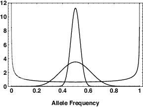
There’s another way of looking at the interaction between drift and mutation. Suppose we have an infinite set of populations with two alleles, \(A_1\) and \(A_2\). Suppose further that the rate of mutation from \(A_1\) to \(A_2\) is equal to the rate of mutation from \(A_2\) to \(A_1\).6 Call that rate \(\mu\). In the absence of mutation a fraction \(p_0\) of the populations would fix on \(A_1\) and the rest would fix on \(A_2\), where \(p_0\) is the original frequency of \(A_1\). With recurrent mutation, no population will ever be permanently fixed for one allele or the other. Instead we see the pattern illustrated in Figure 1
When \(4N\mu < 1\) the stationary distribution of allele frequencies is bowl-shaped, i.e, most populations have allele frequencies near 0 or 1. When \(4N\mu > 1\), the stationary distribution of allele frequencies is hump-shaped, i.e., most populations have allele frequencies near 0.5.7 In other words if the population is “small,” drift dominates the distribution of allele frequencies and causes populations to become differentiated. If the population is “large,” mutation dominates and keeps the allele frequencies in the different populations similar to one another. That’s what we mean when we say that a population is “large” or “small”. A population is “large” if evolutionary processes other than drift have a predominant influence on the outcome. It’s “small” if drift has a predominant role on the outcome.
A population is large with respect to the drift-mutation process if \(4N\mu > 1\), and it is small if \(4N\mu < 1\). Notice that calling a population large or small is really just a convenient shorthand. There isn’t much of a difference between the allele frequency distributions when \(4N\mu = 0.9\) and when \(4N\mu = 1.1\). Notice also that because mutation is typically rare, on the order of \(10^{-5}\) or less per locus per generation for a protein-coding gene, a population must be pretty large (\(> 25,000\)) to be considered large with respect to drift and mutation. Notice also that whether the population is “large” or “small” will depend on the mutation rate at the loci that you’re studying. For example, mutation rates are typically on the order of \(10^{-3}\) for microsatellites. So a population would be “large” with respect to microsatellites if \(N > 250\). Think about what that means. If we had a population with 1000 individuals, it would be “large” with respect to microsatellite evolution and “small” with respect to evolution at a protein-coding locus.
I just pointed out that if populations are isolated from one another they will tend to diverge from one another as a result of genetic drift. Recurrent mutation, which “pushes” all populations towards the same allele frequency, is one way in which that tendency can be opposed. If populations are not isolated, but exchange migrants with one another, then migration will also oppose the tendency for populations to become different from one another. It should be obvious that there will be a tradeoff similar to the one with mutation: the larger the populations, the less the tendency for them to diverge from one another and, therefore, the more migration will tend to make them similar. To explore how drift and migration interact we can use an approach exactly analogous to what we used for mutation.
The model of migration we’ll consider is an extremely oversimplified one. It imagines that every allele brought into a population is different from any of the resident alleles.8 It also imagines that all populations receive the same fraction of migrants. Because any immigrant allele is different, by assumption, from any resident allele we don’t even have to keep track of how far apart populations are from one another, since populations close by will be no more similar to one another than populations far apart. This is Wright’s infinite island model of migration. Given these assumptions, we can write the following: \[f_{t+1} = \left(\left(\frac{1}{2N}\right) + \left(1 - \frac{1}{2N}\right)f_t\right)(1-m)^2 \quad \label{eq:f-m} .\]
That might look fairly familiar. In fact, it’s identical to equation ([eq:f-mu]) except that there’s an \(m\) in ([eq:f-m]) instead of a \(\mu\). \(m\) is the migration rate, the fraction of individuals in a population that is composed of immigrants. More precisely, \(m\) is the backward migration rate. It’s the probability that a randomly chosen individual in this generation came from a population different from the one in which it is currently found in the preceding generation. Normally we’d think about the forward migration rate, i.e., the probability that a randomly chosen individual will go to a different population in the next generation, but backwards migration rates turn out to be more convenient to work with in most population genetic models.9
It shouldn’t surprise you that if equations ([eq:f-mu]) and ([eq:f-m]) are so similar the equilibrium \(f\) under drift and migration is \[\hat f \approx \frac{1}{4Nm + 1}\] In fact, the two allele analog to the mutation model I presented earlier turns out to be pretty similar, too.
If \(2Nm > 1\), the stationary distribution of allele frequencies is hump-shaped, i.e., the populations tend not to diverge from one another.10
If \(2Nm < 1\), the stationary distribution of allele frequencies is bowl-shaped, i.e., the populations tend to diverge from one another.
Now there’s a consequence of these relationships that’s both surprising and odd. \(N\) is the population size. \(m\) is the fraction of individuals in the population that are immigrants. So \(Nm\) is the number of individuals in the population that are new immigrants in any generation. That means that if populations receive more than one new immigrant every other generation, on average, they’ll tend not to diverge in allele frequency from one another.11 It doesn’t make any difference if the populations have a million individuals apiece or ten. One new immigrant every other generation is enough to keep them from diverging.
With a little more reflection, this result is less surprising than it initially seems. After all in populations of a million individuals, drift will be operating very slowly, so it doesn’t take a large proportion of immigrants to keep populations from diverging.12 In populations with only ten individuals, drift will be operating much more quickly, so it takes a large proportion of immigrants to keep populations from diverging.13
These notes are licensed under the Creative Commons Attribution License. To view a copy of this license, visit or send a letter to Creative Commons, 559 Nathan Abbott Way, Stanford, California 94305, USA.