At this point, we’ve refined the neutral theory quite a bit. Our understanding of how molecules evolve now recognizes that some substitutions are more likely than others, but we’re still proceeding under the assumption that most nucleotide substitutions are neutral or detrimental. So far we’ve argued that variation like what Hubby and Lewontin found is not likely to be maintained by natural selection. But we have strong evidence that heterozygotes for the sickle-cell allele are more fit than either homozygote in human populations where malaria is prevalent. That’s an example where selection is acting to maintain a polymorphism, not to eliminate it. Are there other examples? How could we detect them?
In the 1970s a variety of studies suggested that a polymorphism in the locus coding for alcohol dehydrogenase in Drosophila melanogaster might not only be subject to selection but that selection may be acting to maintain the polymorphism. As DNA sequencing became more practical at about the same time,1 population geneticists began to realize that comparative analyses of DNA sequences at protein-coding loci could provide a powerful tool for unraveling the action of natural selection. Synonymous sites within a protein-coding sequence provide a powerful standard of comparison. Regardless of
the demographic history of the population from which the sequences were collected,
the length of time that populations have been evolving under the sample conditions and whether it has been long enough for the population to have reached a drift-migration-mutation-selection equilibrium, or
the actual magnitude of the mutation rate, the migration rate, or the selection coefficients
the synonymous positions within the sequence provide an internal control on the amount and pattern of differentiation that should be expected when substitutions are neutral.2 Thus, if we see different patterns of nucleotide substitution at synonymous and non-synonymous sites, we can infer that selection is having an effect on amino acid substitutions.
Kreitman took advantage of these ideas to provide additional insight into whether natural selection was likely to be involved in maintaining the polymorphism at Adh in Drosophila melanogaster. He cloned and sequenced 11 alleles at this locus, each a little less than 2.4kb in length.3 If we restrict our attention to the coding region, a total of 765bp, there were 6 distinct sequences that differed from one another at between 1 and 13 sites. Given the observed level of polymorphism within the gene, there should be 9 or 10 amino acid differences observed as well, but only one of the nucleotide differences results in an amino acid difference, the amino acid difference associated with the already recognized electrophoretic polymorphism. Thus, there is significantly less amino acid diversity than expected if nucleotide substitutions were neutral, consistent with my assertion that most mutations are deleterious and that natural selection will tend to eliminate them. In other words, another example of the “sledgehammer principle.”
Does this settle the question? Is the Adh polymorphism another example of allelic variants being neutral or selected against? Would I be asking these questions if the answer were “Yes”?
A few years after Kreitman appeared, Kreitman and Aguadé published an analysis in which they looked at levels of nucleotide diversity in the Adh region, as revealed through analysis of RFLPs, in D. melanogaster and the closely related D. simulans. Why the comparative approach? Well, Kreitman and Aguadé remembered that the neutral theory of molecular evolution makes two predictions that are related to the underlying mutation rate:
If mutations are neutral, the substitution rate is equal to the mutation rate.
If mutations are neutral, the diversity within populations should
be about
Thus, if variation at the Adh locus in D. melanogaster is selectively neutral, the amount of divergence between D. melanogaster and D. simulans should be related to the amount of diversity within each. What they found instead is summarized in Table 1.
The expected level of diversity in each part of the Adh locus is calculated assuming that the probability of polymorphism is independent of what position in the locus we are examining.4 Specifically, Kreitman and Aguadé calculated the expected polymorphism as follows:
They calculated the number of “site equivalents” in each region of the locus. A site equivalent is the actual length of the region (in number of nucleotides) times the fraction of changes within that sequence that would lead to gain or loss of a restriction site.5 There were 414 site equivalents in the 5’ flanking region, 411 site equivalents in the Adh locus, and 129 site equivalents in the 3’ flanking region.
They calculated the fraction of site equivalents that were
polymorphic across the entire locus:
They calculated the expected number of polymorphic sites within a region as the product of the number of site equivalents and the fraction of polymorphic site equivalents.
They used the same approach to calculate the expected divergence between D. melanogaster and D. simulans with one important exception. They directly compared the nucleotide sequence of one Adh allele from D. melanogaster with one Adh allele from D. simulans.6 As a result, they didn’t have to use the site equivalent correction. They could directly use the number of nucleotides in each region of the gene.
| 5’ flanking | Adh locus | 3’ flanking | |
|---|---|---|---|
| Diversity |
|||
| Observed | 9 | 14 | 2 |
| Expected | 10.8 | 10.8 | 3.4 |
| Divergence |
|||
| Observed | 86 | 48 | 31 |
| Expected | 55 | 76.9 | 33.1 |
Notice that there is substantially less divergence between D. melanogaster and D. simulans at the Adh locus than would be expected, based on the average level of divergence across the entire region. That’s consistent with the earlier observation that most amino acid substitutions are selected against. On the other hand, there is more nucleotide diversity within D. melanogaster than would be expected based on the levels of diversity seen in across the entire region. What gives?
Time for a trip down memory lane. Remember something called
“coalescent theory?” It told us that for a sample of neutral genes from
a population, the expected time back to a common ancestor for all of
them is about
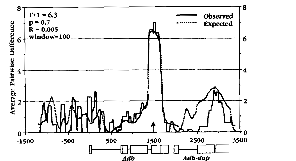
Kreitman and Hudson extended this approach by looking more carefully within the region to see where they could find differences between observed and expected levels of nucleotide sequence diversity. They used a “sliding window” of 100 silent base pairs in their calculations. By “sliding window” what they mean is that first they calculate statistics for bases 1-100, then for bases 2-101, then for bases 3-102, and so on until they hit the end of the sequence (Figure 1).
To me there are two particularly striking things about this figure. First, the position of the single nucleotide substitution responsible for the electrophoretic polymorphism is clearly evident. Second, the excess of polymorphism extends for only a 200-300 nucleotides in each direction. That means that the rate of recombination within the gene is high enough to randomize the nucleotide sequence variation farther away.7
I’ve already mentioned the HapMap project , a collection of genotype data at roughly 3.2M SNPs in the human genome. The data in phase II of the project were collected from four populations:
Yoruba (Ibadan, Nigeria)
Japanese (Tokyo, Japan)
Han Chinese (Beijing, China)
ancestry from northern and western Europe (Utah, USA)
We expect genetic drift to result in allele frequency differences
among populations, and we can summarize the extent of that
differentiation at each locus with
So far we’ve been comparing rates of synonymous and non-synonymous substitution to detect the effects of natural selection on molecular polymorphisms. Tajima proposed a method that builds on the foundation of the neutral theory of molecular evolution in a different way. I’ve already mentioned the infinite alleles model of mutation several times. When thinking about DNA sequences a closely related approximation is to imagine that every time a mutation occurs, it occurs at a different site.9 If we do that, we have an infinite sites model of mutation.
When dealing with nucleotide sequences in a population context there are two statistics of potential interest:
The number of nucleotide positions at which
a polymorphism is found or, equivalently, the number of segregating
sites,
The average number of nucleotide differences between two
sequences,
The quantity
If the variation is neutral and the population is at a drift-mutation
equilibrium, then
Overdominance will allow alleles belonging to the different classes
to become quite divergent from one another.
If the population has recently undergone a bottleneck, then
If there is purifying selection, mutations will occur and accumulate
at silent sites, but they aren’t likely ever to become very common.
Thus, there are likely to be lots of segregating sites, but not much
heterozygosity, meaning that
Similarly, if the population has recently begun to expand, mutations
that occur are unlikely to be lost, increasing
In short,
We have no evidence for changes in population size or for any particular pattern of selection at the locus.16
The population size may be increasing or we may have evidence for purifying selection at this locus.
The population may have suffered a recent bottleneck (or be decreasing) or we may have evidence for overdominant selection at this locus.
If we have data available for more than one locus, we may be able to distinguish changes in population size from selection at any particular locus. After all, all loci will experience the same demographic effects, but we might expect selection to act differently at different loci, especially if we choose to analyze loci with different physiological function.
A quick search in Google Scholar reveals that the paper in which
Tajima described this approach has been cited over 15,000 times.17 Clearly it has been widely used for
interpreting patterns of nucleotide sequence variation. Although it is a
very useful statistic, Zeng et al. point out that there are important
aspects of the data that Tajima’s
We’ve seen that both drift and natural selection can lead to allele
frequency changes in a population. Is there any way to tell how much of
the allele frequency change in a population is a result of natural
selection?18 Well, to do so we need a set of
allele frequencies measured at many loci at several different time
steps. With that we can define
These notes are licensed under the Creative Commons Attribution License. To view a copy of this license, visit or send a letter to Creative Commons, 559 Nathan Abbott Way, Stanford, California 94305, USA.