The study of evolutionary biology is commonly divided into two components: study of the processes by which evolutionary change occurs and study of the patterns produced by those processes. By “pattern” we mean primarily the pattern of phylogenetic relationships among species or genes.1 Studies of evolutionary processes often don’t often devote too much attention to evolutionary patterns, except insofar as it is often necessary to take account of evolutionary history in determining whether or not a particular feature is an adaptation. Similarly, studies of evolutionary pattern sometimes try not to use any knowledge of evolutionary processes to improve their guesses about phylogenetic relationships, because the relationship between process and pattern can be tenuous.2 Those who take this approach argue that invoking a particular evolutionary process seems often to be a way of making sure that you get the pattern you want to get from the data.
Or at least that’s the way it was in evolutionary biology when evolutionary biologists were concerned primarily with the evolution of morphological, behavioral, and physiological traits and when systematists used primarily anatomical, morphological, and chemical features (but not proteins or DNA) to describe evolutionary patterns. With the advent of molecular biology after the Second World War and its application to an increasing diversity of organisms in the late 1950s and early 1960s, that began to change. Goodman used the degree of immunological cross-reactivity between serum proteins as an indication of the evolutionary distance among primates. Zuckerkandl and Pauling proposed that after species diverged, their proteins diverged according to a “molecular clock,” suggesting that molecular similarities could be used to reconstruct evolutionary history. In 1966, Harris and Lewontin and Hubby showed that human populations and populations of Drosophila pseudoobscura respectively, contained surprising amounts of genetic diversity.
We’ll focus first on advances made in understanding the processes of molecular evolution. Once we have a passing understanding of those processes, we’ll shift to topics that are generally more interesting to evolutionary biologists, i.e., making inferences about evolutionary patterns from molecular data. Up to this point in the course we’ve completely ignored evolutionary pattern.3 As you’ll see in what follows, however, any discussion of molecular evolution, even if it focuses on understanding the processes, cannot avoid some careful attention to the pattern.
If you’re interested in the history of molecular evolution, you may be interested in this review of the types of data that population geneticists have used in the last 50 or 60 years to provide insights into evolutionary processes. If you’re not interested in the history, feel free to skip this section. I will touch on only a couple of the real high points during lecture. Much of the data being collected now for population genetics is treated as single nucleotide polymorphisms (sometimes with genetic linkage taken into account) or copy-number variation, and it is derived either from low-coverage whole-genome resequencing or from a reduced representation sequencing approach like some version of RADseq or genotyping-by-sequencing. The exceptions are that for some purposes, microsatellites are still the marker of choice and for others, RNAseq can be used to explore differences in gene expression between individuals or under different conditions.
We’ve already encountered a couple of these (microsatellites and SNPs), but there are a variety of important categories into which we can group data used for molecular evolutionary analyses. Even though studies of molecular evolution in the last 20-25 years have focused mostly on data derived from DNA sequence or copy number variation, modern applications of molecular data evolved from earlier applications. Markers that were used before the advent of (relatively) easy and cheap DNA sequencing had their limitations, but analyses of those data also laid the groundwork for most or all of what’s going on in analyses of molecular evolution today. Thus, it’s useful to remind everyone what kinds of molecular data have been used to provide insight into evolutionary patterns and processes and to agree on some terminology for the ones we’ll say something about. Let’s talk first about the physical basis of the underlying data. Then we’ll talk about the laboratory methods used to reveal variation.
With the exception of RNA viruses, the hereditary information in all organisms is carried in DNA. Ultimately, differences in any of the molecular markers we study (and of genetically-based morphological, behavioral, or physiological traits) is associated with some difference in the physical structure of DNA.
A difference in nucleotide sequence is the most obvious way in which two homologous stretches of DNA may differ. The differences may be in translated portions of protein genes (exons), portions of protein genes that are transcribed but not translated (e.g., introns, 5’ or 3’ untranslated regions), non-transcribed functional regions (e.g., promoters), or regions without apparent function.
Because of redundancy in the genetic code, a difference in nucleotide sequence at a protein-coding locus may or may not result in proteins with a different amino acid sequence. Important note: Don’t forget that some loci code for RNA that has an immediate function without being translated to a protein, e.g., ribosomal RNA and various small nuclear RNAs.
Differences in amino acid sequence may or may not lead to a different distribution of \(\alpha\)-helices and \(\beta\)-sheets, to a different three-dimensional structure, or to different multisubunit combinations.
At certain loci in some organisms the expression pattern of a particular allele depends on whether that allele was inherited from the individual’s father or its mother.
Functional differences among individuals may arise because of differences in the patterns of gene expression, even if there are no differences in the primary sequences of the genes that are expressed.4
Particular genes may differ between organisms because of differences in the position and number of introns. At the whole genome level, there may be differences in the amount and kind of repetitive sequences, in the amount and type of sequences derived from transposable elements, in the relative proportion of G-C relative to A-T, or even in the identity and arrangement of genes that are present. In microbial species, only a subset of genes are present in all strains. For example, in Streptococcus pneumoniae the “core genome” contains only 73% of the loci present in one fully sequenced reference strain . Similarly, a survey of 20 strains of Escherichia coli and one of E. fergusonii, E. coli’s closest relative, identified only 2000 homologous loci that were present in all strains out of 18,000 orthologous loci identified
Even within diploid genomes, there may be substantial differences in the number of copies of particular genes. In humans, for example, 76 copy-number polymorphisms (CNPs) were identified in a sample of only 20 individuals, and individuals differed from one another by an average of 11 CNPs. .
It is worth remembering that in nearly all eukaryotes there are two different genomes whose characteristics may be analyzed: the nuclear genome and the mitochondrial genome. In plants there is a third: the chloroplast genome. In some protists, there may be even more, because of secondary or tertiary endosymbiosis. The mitochondrial and chloroplast genomes are typically inherited only through the maternal line, although some instances of biparental inheritance are known.5 In conifers, chloroplasts are paternally inherited, i.e., through the pollen parent, and mitochondria are maternally inherited, i.e., through the seed parent
The diversity of laboratory techniques used to reveal molecular variation is even greater than the diversity of underlying physical structures. Various techniques involving direct measurement of aspects of DNA sequence variation are by far the most common today, so I’ll mention only a few of the techniques that were most widely used in the past.6
Some molecules, notably protein molecules, induce an immune response in common laboratory mammals. The extent of cross-reactivity between an antigen raised to humans and chimps, for example, can be used as a measure of evolutionary distance. The immunological distance between humans and chimps is smaller than it is between humans and orangutans, suggesting that humans and chimps share a more recent common ancestor.
Once repetitive sequences of DNA have been “subtracted out”,7 the rate and temperature at which DNA species from two different species anneal reflects the average percent sequence divergence between them. The percent sequence divergence can be used as a measure of evolutionary distance. Immunological distances and DNA-DNA hybridization were once widely used to identify phylogenetic relationships among species. Neither is now widely used in molecular evolution studies.
Biochemists recognized in the late 1950s that many soluble enzymes occurred in multiple forms within a single individual. Population geneticists, notably Hubby and Lewontin, later recognized that in many cases, these different forms corresponded to different alleles at a single locus, allozymes. Allozymes are relatively easy to score in most macroscopic organisms, they are typically co-dominant (the allelic composition of heterozygotes can be inferred), and they allow investigators to identify both variable and non-variable loci.8 Patterns of variation at allozyme loci may not be representative of genetic variation that does not result from differences in protein structure or that are related to variation in proteins that are insoluble.
In the 1970s molecular geneticists discovered restriction enzymes, enzymes that cleave DNA at specific 4, 5, or 6 base pair sequences, the recognition site. A single nucleotide change in a recognition site is usually enough to eliminate it. Thus, presence or absence of a restriction site at a particular position in a genome provides compelling evidence of an underlying difference in nucleotide sequence at that positon.
With the advent of the polymerase chain reaction in the late 1980s, several related techniques were developed for the rapid assessment of genetic variation in organisms for which little or no prior genetic information was available. These methods differ in details of how the laboratory procedures are performed, but they are similar in that they (a) use PCR to amplify anonymous stretches of DNA, (b) generally produce larger amounts of variation than allozyme analyses of the same taxa, and (c) are bi-allelic, dominant markers. They have the advantage, relative to allozymes, that they sample more or less randomly through the genome. They have the disadvantage that heterozygotes cannot be distinguished from dominant homozygotes, meaning that it is difficult to use them to obtain information about levels of within population inbreeding.9
Satellite DNA, highly repetitive DNA associated with heterochromatin, had been known since biochemists first began to characterize the large-scale structure of genomes in DNA-DNA hybridization studies. In the mid-late 1980s several investigators identified smaller repetitive units dispersed throughout many genomes. Microsatellites, which consist of short (2-6) nucleotide sequences repeated many times, have proven particularly useful for analyses of variation within populations since the mid-1990s.10 Because of high mutation rates at each locus, they commonly have many alleles. Moreover, they are typically co-dominant, making them more generally useful than dominant markers. Identifying variable microsatellite loci is, however, more laborious than identifying AFLPs, RAPDs, or ISSRs.
The advent of automated sequencing11 has greatly increased the amount of population-level data available on nucleotide sequences. The even more recent arrival of high-throughput DNA sequencing means that sequence information is accumulating even more rapidly. Nucleotide sequence data has an important advantage over most of the types of data discussed so far: allozymes, RFLPs, AFLPs, RAPDs, and ISSRs all hide some amount of nucleotide sequence variation. Nucleotide sequence differences need not be reflected in any of those markers. On the other hand, each of those markers provides information on variation at several or many, independently inherited loci. Nucleotide sequence information reveals differences at a location that rarely extends more than 2-3kb. Of course, as next generation sequencing techniques become less expensive and more widely available, we will see more and more examples of nucleotide sequence variation from many loci within individuals.12
In organisms that are genetically well-characterized, it is possible to identify a large number of single nucleotide positions that harbor polymorphisms. SNPs potentially provide high-resolution insight into patterns of variation within the genome. For example, the HapMap project identified approximately 3.2M SNPs in the human genome, or about one every kb . With the advent of RAD-seq, GBS, and similar approaches, it has become possible to identify large numbers of SNPs even in organisms that are not genetically well-characterized .
As you can see from these brief descriptions, each of the markers reveals different aspects of underlying hereditary differences among individuals, populations, or species. There is no single “best” marker for evolutionary analyses. Which is best depends on the question you are asking. In many cases in molecular evolution, the interest is intrinsically in the evolution of the molecule itself, so the choice is based not on what those molecules reveal about the organism that contains them but on what questions about which molecules are the most interesting.
Underlying much of what we’re going to discuss in this part of the course is the idea that we should be able to describe the degree of difference between nucleotide sequences, proteins, or anything else as a result of some underlying evolutionary processes. To illustrate the principle, let’s start with nucleotide sequences and develop a fairly simple model that describes how they become different over time.13
Let \(q_t\) be the probability that two homologous nucleotides are identical after having been evolving for \(t\) generations independently since the gene in which they were found was replicated in their common ancestor. Let \(\lambda\) be the probability of a substitution14 occuring at this nucleotide position in either of the two genes during a small time interval, \(\Delta t\). Then \[\begin{aligned} q_{t+\Delta t} &=& (1 - \lambda\Delta t)^2q_t + 2\left(1 - \lambda\Delta t\right)\left({1 \over 3}\lambda\Delta t\right)(1 - q_t) + \hbox{o}(\Delta t^2) \\ &=& (1 - 2\lambda\Delta t)q_t + \left({2 \over 3}\lambda \Delta t\right) (1 - q_t) + \hbox{o}(\Delta t^2) \\ q_{t+\Delta t} - q_t &=& {2 \over 3}\lambda\Delta t - {8 \over 3}\lambda\Delta tq_t + \hbox{o}(\Delta t^2) \\ {q_{t+\Delta t} - q_t \over \Delta t} &=& {2 \over 3}\lambda - {8 \over 3}\lambda q_t + \hbox{o}(\Delta t) \\ \lim_{\Delta t\to 0}{q_{t+\Delta t} - q_t \over \Delta t} = {dq_t \over dt} &=& {2 \over 3}\lambda - {8 \over 3}\lambda q_t \\ & \mbox{TAMO} & \\ q_t &=& 1 - {3 \over 4}\left(1 - e^{-8\lambda t/3}\right) \\ \end{aligned}\] The expected number of nucleotide substitutions separating the two sequences at any one position since they diverged is \(d = 2\lambda t\).15 Thus, \[\begin{aligned} q_t &=& 1 - {3 \over 4}\left(1 - e^{-4d/3}\right) \\ d &=& -{3 \over 4}\ln\left[1 - {4 \over 3}(1 - q_t)\right] \\ \end{aligned}\] This is the simplest model of nucleotide substitution possiblethe Jukes-Cantor model . It assumes
that substitutions are equally likely at all positions and
that substitution among all nucleotides is equally likely.
Let’s examine the second of those assumptions first. Observed differences between nucleotide sequences shows that some types of substitutions, i.e., transitions (\(A \iff G\) [purine to purine], \(C \iff T\) [pyrimidine to pyrimidine]), occur much more frequently than others, i.e., transversions (\(A \iff T\), \(A \iff C\), \(G \iff C\), \(G \iff T\) [purine to pyrimidine or vice versa]). There are a variety of different substitution models corresponding to different assumed patterns of substitution: Kimura 2 parameter (K2P), Felsenstein 1984 (F84), Hasegawa-Kishino-Yano 1985 (HKY85), Tamura and Nei (TrN), and generalized time-reversible (GTR). The GTR is, as its name suggests, the most general time-reversible model. It allows substitution rates to differ between each pair of nucleotides. That’s why it’s general. It still requires, however, that the substitution rate be the same in both directions. That’s what it means to say that it’s time reversible. While it is possible to construct a model in which the substitution rate differs depending on the direction of substitution, it leads to something of a paradox: with non-reversible substitution models the distance between two sequences \(A\) and \(B\) depends on whether we measure the distance from \(A\) to \(B\) or from \(B\) to \(A\). That is to say that the distance from \(A\) to \(B\) isn’t the same as the distance from \(B\) to \(A\).
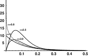
There are two ways in which the rate of nucleotide substitution can be allowed to vary from position to positionthe phenomenon of among-site rate variation. First, we expect the rate of substitution to depend on codon position in protein-coding genes. The sequence can be divided into first, second, and third codon positions and rates calculated separately for each of those positions. Second, we can assume a priori that there is a distribution of different rates possible and that this distribution is described by one of the standard distributions from probability theory. We then imagine that the substitution rate at any given site is determined by a random draw from that probability distribution. The gamma distribution is widely to describe the pattern of among-site rate variation, because it can approximate a wide variety of different distributions (Figure 1).16
The mean substitution rate in each curve above is 0.1. The curves differ only in the value of a parameter, \(\alpha\), called the “shape parameter.” The shape parameter gives a nice numerical description of how much rate variation there is, except that it’s backwards. The larger the parameter, the less among-site rate variation there is.
I didn’t make a big deal of it in what we just went over, but in deriving the Jukes-Cantor equation I used the phrase “substitution rate” instead of the phrase “mutation rate.”17 As a preface to what is about to follow, let me explain the difference.
Mutation rate refers to the rate at which changes are incorporated into a nucleotide sequence during the process of replication, i.e., the probability that an allele differs from the copy of that allele in its parent from which it was derived. Mutation rate refers to the rate at which mutations arise.
An allele substitution occurs when a newly arisen allele is incorporated into a population, e.g., when a newly arisen allele becomes fixed in a population. Substitution rate refers to the rate at which allele substitutions occur.
Mutation rates and substitution rates are obviously relatedsubstitutions can’t happen unless mutations occur, after all, but it’s important to remember that they refer to different processes.
By the early 1960s amino acid sequences of hemoglobins and cytochrome c for many mammals had been determined. When the sequences were compared, investigators began to notice that the number of amino acid differences between different pairs of mammals seemed to be roughly proportional to the time since they had diverged from one another, as inferred from the fossil record. Zuckerkandl and Pauling proposed the molecular clock hypothesis to explain these results. Specifically, they proposed that there was a constant rate of amino acid substitution over time. Sarich and Wilson used the molecular clock hypothesis to propose that humans and apes diverged approximately 5 million years ago. While that proposal may not seem particularly controversial now, it generated enormous controversy at the time, because at the time many paleoanthropologists interpreted the evidence to indicate humans diverged from apes as much as 30 million years ago.
One year after Zuckerkandl and Pauling’s paper, Harris and Hubby and Lewontin showed that protein electrophoresis could be used to reveal surprising amounts of genetic variability within populations. Harris studied 10 loci in human populations, found three of them to be polymorphic, and identified one locus with three alleles. Hubby and Lewontin studied 18 loci in Drosophila pseudoobscura, found seven to be polymorphic, and five that had three or more alleles.
Both sets of observations posed real challenges for evolutionary geneticists. It was difficult to imagine an evolutionary mechanism that could produce a constant rate of substitution. It was similarly difficult to imagine that natural selection could maintain so much polymorphism within populations. The “cost of selection,” as Haldane called it would simply be too high.
Kimura and King and Jukes proposed a way to solve both empirical problems. If the vast majority of amino acid substitutions are selectively neutral,18 then substitutions will occur at approximately a constant rate (assuming that substitution rates don’t vary over time) and it will be easy to maintain lots of polymorphism within populations because there will be no cost of selection. I’ll develop both of those points in a bit more detail in just a moment, but let me first be precise about what the neutral theory of molecular evolution actually proposes. More specifically, let me first be precise about what it does not propose. I’ll do so specifically in the context of protein evolution for now, although we’ll broaden the scope later.
The neutral theory asserts that alternative alleles at variable protein loci are selectively neutral. This does not mean that the locus is unimportant, only that the alternative alleles found at this locus are selectively neutral.
Glucose-phosphate isomerase is an esssential enzyme. It catalyzes the first step of glycolysis, the conversion of glucose-6-phosphate into fructose-6-phosphate.
Natural populations of many, perhaps most, populations of plants and animals are polymorphic at this locus, i.e., they have two or more alleles with different amino acid sequences.
The neutral theory asserts that the alternative alleles are essentially equivalent in fitness, in the sense that genetic drift, rather than natural selection, dominates the dynamics of frequency changes among them.
By selectively neutral we do not mean that the alternative alleles have no effect on physiology or fitness. We mean that the selection among different genotypes at this locus is sufficiently weak that the pattern of variation is determined primarily by the interaction of mutation, drift, mating system, and migration. This is roughly equivalent to saying that \(N_es < 1\), where \(N_e\) is the effective population size and \(s\) is the selection coefficient on alleles at this locus.
Experiments in Colias butterflies, and other organisms have shown that different electrophoretic variants of GPI have different enzymatic capabilities and different thermal stabilities. In some cases, these differences have been related to differences in individual performance.
If populations of Colias are large and the differences in fitness associated with differences in genotype are large, i.e., if \(N_es > 1\), then selection plays a predominant role in determining patterns of diversity at this locus, i.e., the neutral theory of molecular evolution would not apply.
If populations of Colias are small or the differences in fitness associated with differences in genotype are small, or both, then drift plays a predominant role in determining patterns of diversity at this locus, i.e., the neutral theory of molecular evolution applies.
In short, the neutral theory of molecular really asserts only that observed amino acid substitutions and polymorphisms are effectively neutral, not that the loci involved are unimportant or that allelic differences at those loci have no effect on fitness.
We’re now going to calculate the rate of molecular evolution, i.e., the rate of allelic substitution, under the hypothesis that mutations are selectively neutral.19 To get that rate we need two things: the rate at which new mutations occur and the probability with which new mutations are fixed. In a word equation \[\begin{aligned} \mbox{\# of substitutions/generation} &=& (\mbox{\# of mutations/generation})\times(\mbox{probability of fixation}) \\ \lambda &=& \mu_0p_0 \quad . \end{aligned}\] Surprisingly,20 it’s pretty easy to calculate both \(\mu_0\) and \(p_0\) from first principles.
In a diploid population of size \(N\), there are \(2N\) gametes. The probability that any one of them mutates is just the mutation rate, \(\mu\), so \[\mu_0 = 2N\mu \quad . \label{eq:mu-0}\] To calculate the probability of fixation, we have to say something about the dynamics of alleles in populations. Let’s suppose that we’re dealing with a single population, to keep things simple. Now, you have to remember a little of what you learned about the properties of genetic drift. If the current frequency of an allele is \(p_0\), what’s the probability that is eventually fixed? \(p_0\). When a new mutation occurs there’s only one copy of it,21 so the frequency of a newly arisen mutation is \(1/2N\) and \[p_0 = \frac{1}{2N} \quad . \label{eq:p-0}\] Putting ([eq:mu-0]) and ([eq:p-0]) together we find \[\begin{aligned} \lambda &=& \mu_0p_0 \\ &=& (2N\mu)\left(\frac{1}{2N}\right) \\ &=& \mu \quad . \end{aligned}\] In other words, if mutations are selectively neutral, the substitution rate is equal to the mutation rate. Since mutation rates are (mostly) governed by physical factors that remain relatively constant, mutation rates should remain constant, implying that substitution rates should remain constant if substitutions are selectively neutral. In short, if mutations are selectively neutral, we expect a molecular clock.
Protein-coding genes consist of hundreds or thousands of nucleotides, each of which could mutate to one of three other nucleotides.22 That’s not an infinite number of possibilities, but it’s pretty large.23 It suggests that we could treat every mutation that occurs as if it were completely new, a mutation that has never been seen before and will never be seen again. Does that description ring any bells? Does the infinite alleles model sound familiar? It should, because it exactly fits the situation I’ve just described.
Having remembered that this situation is well described by the infinite alleles model, I’m sure you’ll also remember that we can calculate the equilibrium inbreeding coefficient for the infinite alleles model, i.e., \[f = \frac{1}{4N_e\mu + 1} \quad .\] What’s important about this for our purposes, is that to the extent that the infinite alleles model is appropriate for molecular data, then \(f\) is the frequency of homozygotes we should see in populations and \(1-f\) is the frequency of heterozygotes. So in large populations we should find more diversity than in small ones, which is roughly what we do find. Notice, however, that here we’re talking about heterozygosity at individual nucleotide positions,24 not heterozygosity of halpotypes.
In broad outline then, the neutral theory does a pretty good job of dealing with at least some types of molecular data. I’m sure that some of you are already thinking, “But what about third codon positions versus first and second?” or “What about the observation that histone loci evolve much more slowly than interferons or MHC loci?” Those are good questions, and those are where we’re going next. As we’ll see, molecular evolutionists have elaborated the framework extensively25 in the last sixty years, but these basic principles underlie every investigation that’s conducted. That’s why I wanted to spend a fair amount of time going over the logic and consequences. Besides, it’s a rare case in population genetics where the fundamental mathematics that lies behind some important predictions are easy to understand.26
These notes are licensed under the Creative Commons Attribution License. To view a copy of this license, visit or send a letter to Creative Commons, 559 Nathan Abbott Way, Stanford, California 94305, USA.