We’ve already encountered \(\pi\), the nucleotide diversity in a population, namely \[\pi = \sum_{ij} x_ix_j \delta_{ij} \quad ,\] where \(x_i\) is the frequency of the \(i\)th haplotype and \(\delta_{ij}\) is the fraction of nucleotides at which haplotypes \(i\) and \(j\) differ.1 It shouldn’t come to any surprise to you that just as there is interest in partitioning diversity within and among populations when we’re dealing with simple allelic variation, i.e., Wright’s \(F\)-statistics, there is interest in partitioning diversity within and among populations when we’re dealing with nucleotide sequence or other molecular data. The approach I’m going to describe is known as Analysis of Molecular VAriance (AMOVA) . We’ll see later that AMOVA can be used very generally to partition variation when there is a distance we can use to describe how different alleles are from one another, but for now, let’s stick with nucleotide sequence data and think of \(\delta_{ij}\) simply as the fraction of nucleotide sites at which two sequences differ.
The notation now becomes just a little bit more complicated. We will now use \(x_{ik}\) to refer to the frequency of the \(i\)th haplotype in the \(k\)th population. Then \[x_{i\cdot} = \frac{1}{K}\sum_{k=1}^K x_{ik}\] is the mean frequency of haplotype \(i\) across all populations, where \(K\) is the number of populations. We can now define \[\begin{aligned} \pi_t &=& \sum_{ij} x_{i\cdot}x_{j\cdot} \delta_{ij} \\ \pi_s &=& \frac{1}{K}\sum_{k=1}^K\sum_{ij} x_{ik}x_{jk}\delta_{ij} \quad , \end{aligned}\] where \(\pi_t\) is the nucleotide sequence diversity across the entire set of populations and \(\pi_s\) is the average nucleotide sequence diversity within populations. Then we can define \[\Phi_{st} = \frac{\pi_t - \pi_s}{\pi_t} \quad , \label{eq:phi-st}\] which is the direct analog of Wright’s \(F_{st}\) for nucleotide sequence diversity. Why? Well, that requires you to remember stuff we covered about two months ago.
To be a bit more specific, refer back to the notes on \(F_{ST}\).2. When you do, you’ll see that we defined \[F_{IT} = 1 - \frac{H_i}{H_t} \quad ,\] where \(H_i\) is the average heterozygosity in individuals and \(H_t\) is the expected panmictic heterozygosity. Defining \(H_s\) as the average panmictic heterozygosity within populations, we then observed that \[\begin{aligned} 1 - F_{IT} &=& \frac{H_i}{H_t} \\ &=& \frac{H_i}{H_s}\frac{H_s}{H_t} \\ &=& (1 - F_{IS})(1 - F_{ST}) \quad . \end{aligned}\] We can rearrange that equation a bit to solve for \(F_{ST}\) in terms of \(F_{IT}\) and \(F_{IS}\).
\[\begin{aligned} 1-F_{ST} &=& \frac{1-F_{IT}}{1-F_{IS}} \\ F_{ST} &=& \frac{\left(1-F_{IS}\right)-\left(1-F_{IT}\right)}{1-F_{IS}} \\ &=& \frac{\left(H_i/H_s\right) - \left(H_i/H_t\right)}{H_i/H_s} \\ &=& \frac{\left(1/H_s\right) - \left(1/H_t\right)}{1/H_s} \\ &=& 1 - \frac{1/H_t}{1/H_S} \\ &=& 1 - \frac{H_s}{H_t} \quad . \end{aligned}\] In short, another way to think about \(F_{ST}\) is \[F_{ST} = \frac{H_t - H_s}{H_t} \quad . \label{eq:f-st}\] Now if you compare equation ([eq:phi-st]) and equation ([eq:f-st]), you’ll see the analogy.
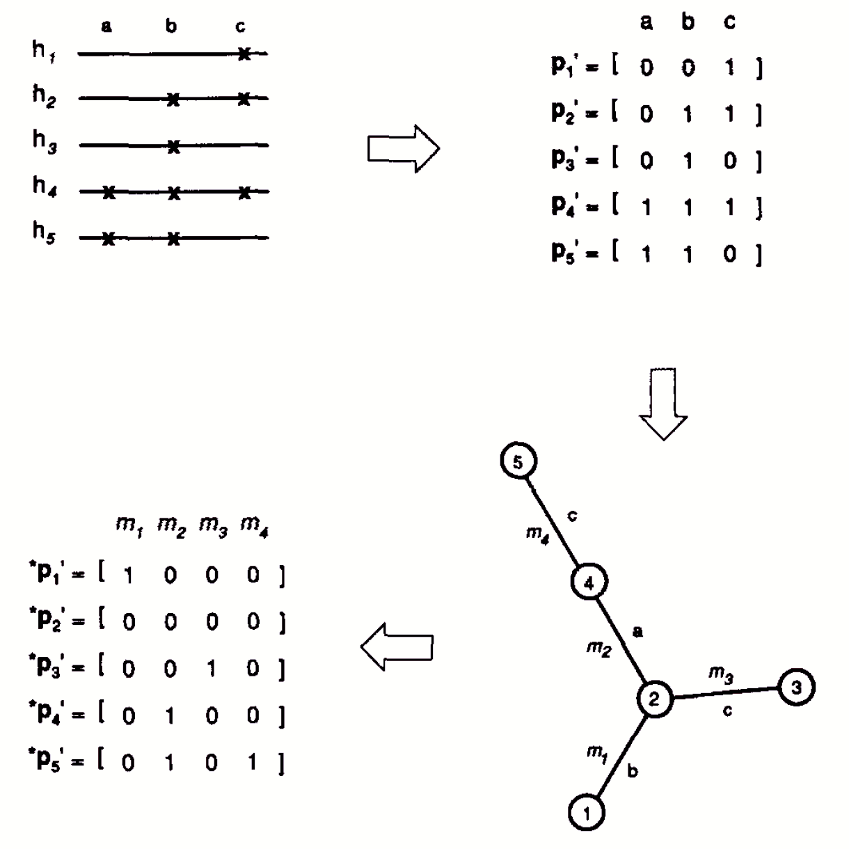
So far I’ve motivated this approach by thinking about \(\delta_{ij}\) as the fraction of sites at which two haplotypes differ and \(\pi_s\) and \(\pi_t\) as estimates of nucleotide diversity. But nothing in the algebra leading to equation ([eq:phi-st]) requires that assumption. Excoffier et al. pointed out that other types of molecular data can easily be fit into this framework. We simply need an appropriate measure of the “distance” between different haplotypes or alleles. Even with nucleotide sequences the appropriate \(\delta_{ij}\) may reflect something about the mutational pathway likely to connect sequences rather than the raw number of differences between them. For example, the distance might be a Jukes-Cantor distance or a more general distance measure that accounts for more of the properties we know are associated with nucleotide substitution. The idea is illustrated in Figure 1.
Notice that when we’re partitioning diversity with AMOVA, we’re using the word “diversity” in a different sense than we did with \(F\)-statistics. With \(F\)-statistics we were thinking about diversity solely in terms of allele frequency differences. With AMOVA we’re thinking about diversity in terms of a combination of haplotype frequency differences and a measure of how differenthow distant those haplotypes are from one another.
Once we have \(\delta_{ij}\) for all pairs of haplotypes or alleles in our sample, we can use the ideas lying behind equation ([eq:phi-st]) to partition diversitythe average distance between randomly chosen haplotypes or allelesinto within and among population components.3 This procedure for partitioning diversity in molecular markers is referred to as an analysis of molecular variance or AMOVA (by analogy with the ubiquitous statistical procedure analysis of variance, ANOVA). Like Wright’s \(F\)-statistics, the analysis can include several levels in the hierarchy.
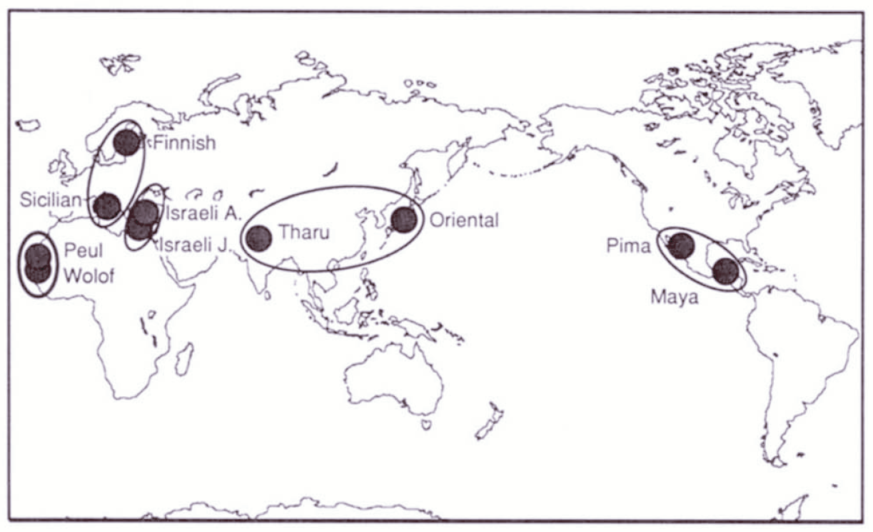
Excoffier et al. illustrate the approach by presenting an analysis of restriction haplotypes in human mtDNA. They analyze a sample of 672 mitochondrial genomes representing two populations in each of five regional groups (Figure 2). They identified 56 haplotypes in that sample. A minimum spanning tree illustrating the relationships and the relative frequency of each haplotype is presented in Figure 3.
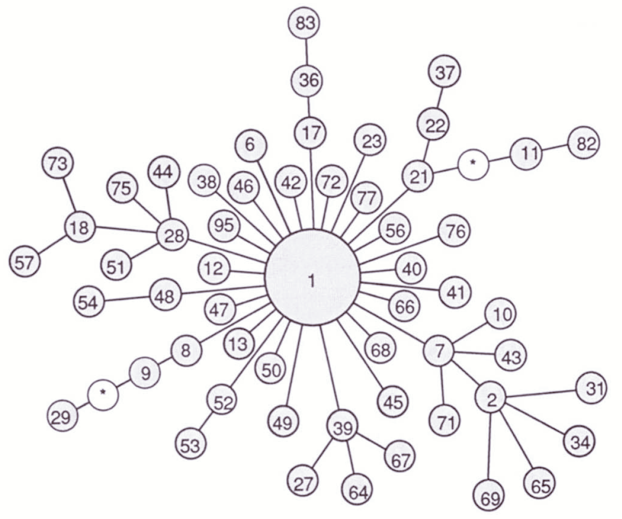
It’s apparent from Figure 3 that haplotype 1 is very common. In fact, it is present in substantial frequency in every sampled population. An AMOVA using the minimum spanning network in Figure 3 to measure distance produces the results shown in Table 1. Notice that there is relatively little differentiation among populations within the same geographical region (\(\Phi_{SC} = 0.044\)). There is, however, substantial differentiation among regions (\(\Phi_{CT} = 0.220\)). In fact, differences among populations in different regions is responsible for nearly all of the differences among populations (\(\Phi_{ST} = 0.246\)).
Remembering that AMOVA partitions a combination of haplotype frequency differences and haplotype differences, the interpretation of the \(\Phi\)-statistics is a little different from the interpretation of \(F\)-statistics. When we say that there is relatively little differentiation among populations within regions and that differences among populations are responsible for most of the among population differences, we mean that the evolutionary distance4 between any two haplotypes from populations within the same region is relatively small while the evolutionary distance between haplotypes from different regions is relatively large. And by “evolutionary distance” we mean both the distance between haplotypes reflected in \(\delta_{ij}\) and the distance due to the extra time it takes haplotypes from different populations to trace their ancestry back to the same population.
Notice also that \(\Phi\)-statistics follow the same rules as Wright’s \(F\)-statistics, namely \[\begin{aligned} 1 - \Phi_{ST} &=& (1 - \Phi_{SC})(1 - \Phi_{CT}) \\ 0.754 &=& (0.956)(0.78) \quad , \end{aligned}\] within the bounds of rounding error.5
| Component of differentiation | \(\Phi\)-statistics |
|---|---|
| Among regions | \(\Phi_{CT} = 0.220\) |
| Among populations within regions | \(\Phi_{SC} = 0.044\) |
| Among all populations | \(\Phi_{ST} = 0.246\) |
When we were discussing the coalescent in structured populations, you may recall that I pointed out that there is a relationship between \(F_{ST}\) and coalescent times.6 Specifically, Slatkin pointed out that if mutation is rare then \[F_{ST} \approx \frac{\bar t - \bar t_0}{\bar t} \quad ,\] where \(\bar t\) is the average time to coalescence for two genes drawn at random without respect to population and \(\bar t_0\) is the average time to coalescence for two genes drawn at random from the same populations. Results in show that when \(\delta_{ij}\) is linearly proportional to the time since two sequences have diverged, \(\Phi_{ST}\) is a good estimator of \(F_{ST}\) when \(F_{ST}\) is thought of as a measure of the relative excess of coalescence time resulting from dividing a species into several population. In other words if \(\delta_{ij}\) is a good measure of the evolutionary distance between sequences in the sense that it is directly proportional to the time since the sequences diverged, then the combination of haplotype frequency differences and evolutionary distances among haplotypes may provide insight into the evolutionary relationships among populations of the same species. For yet another way of saying it, if \(\delta_{ij}\) is proportion to divergence time, then \(\phi_{ST}\) tells us how much longer we have to wait for haplotypes to coalesce as a result of the population being subdivided.
These notes are licensed under the Creative Commons Attribution License. To view a copy of this license, visit or send a letter to Creative Commons, 559 Nathan Abbott Way, Stanford, California 94305, USA.