One approach to understanding more about the genetics of quantitative traits takes advantage of the increasing number of genetic markers available as a result of recent advances in molecular genetics. Suppose you have two inbred lines that differ in a trait that interests you, say body weight or leaf width. Call one of them the “high” line and the other the “low” line.1 Further suppose that you have a whole bunch of molecular markers that differ between the two lines, and designate the genotype in the “high” line \(A_1A_1\) and the genotype in the low line \(A_2A_2\).2 One last supposition: Suppose that at loci influencing the phenotype you’re studying the genotype in the “high” line is \(Q_1Q_1\) and the genotype in the “low” line is \(Q_2Q_2\). Each of these loci is what we call a quantitative trait locus or QTL. Now do the following experiment:
Cross the “high” line and the “low” line to construct an \(F_1\).
Intercross individuals in the \(F_1\) generation to form an \(F_2\).3
“Walk” through the genome4 calculating a likelihood score for a QTL at a particular map position, using what we know about the mathematics of recombination rates and Mendelian genetics. In calculating the likelihood score we maximize the likelihood of the data assuming that there is a QTL at this position and estimating the corresponding additive and dominance effects of the allele. We then identify QTLs as those loci where there are “significant” peaks in the map of likelihood scores.
The result is a genetic map showing where QTLs are in the genome and indicating the magnitude of their additive and dominance effects.
QTL mapping is wonderfulprovided that you’re working with an organism where it’s possible to design a breeding program and where the information derived from that breeding program is relevant to variation in natural populations. Think about it. If we do a QTL analysis based on segregation in an \(F_2\) population derived from two inbred lines, all we really know is which loci are associated with phenotypic differences between those two lines. Typically what we really want to know, if we’re evolutionary biologists, is which loci are associated with phenotypic differences between individuals in the population we’re studying. That’s where association mapping comes in. We look for statistical associations between phenotypes and genotypes across a whole population. We expect there to be such associations, if we have a dense enough map, because some of our marker loci will be closely linked to loci responsible for phenotypic variation.
So how does association mapping work? There are two broad approaches, one that is used in genome-wide association studies (GWAS) that is analogous to QTL mapping and one that looks for differences between “cases,” those that exhibit a particular phenotype of interest (e.g., a disease state in humans), and “controls,” those that don’t exhibit the phenotype of interest. Let’s talk about GWAS first.
Imagine that we have a well-mixed population segregating both for a lot of molecular markers spread throughout the genome and for loci influencing a trait we’re interested in, like body weight or leaf width. Let’s call our measurement of that trait \(z_i\) in the \(i\)th individual. Let \(x_{ij}\) be the genotype of individual \(i\) at the \(j\)th locus.5 Then to do association mapping, we simply fit the following regression model: \[y_i = x_{ij}\beta_j + \epsilon_{ij} \quad ,\] where \(\epsilon_{ij}\) is the residual error in our regression estimate and \(\beta_j\) is our estimate of the effect of substituting one allele for another at locus \(j\), i.e., the additive effect of an allele at locus \(j\).6 If \(\beta_j\) is significantly different from 0, we have evidence that there is a locus linked to this marker that influences the phenotype we’re interested in, and we have an estimate of the additive effect of the alleles at that locus.
Notice that I claimed we have evidence that the locus is linked. That’s a bit of sleight of hand. I’ve glossed over something very important. What we have direct evidence for is only that the locus is associated with the phenotype differences. As we’ll see in just a bit, the observed association might reflect physical linkage between the marker locus and a locus influencing the phenotype or it could reflect a statistical association that arises for other reasons, including population structure. So in practice the regression model we fit is a more complicated than the one I just described. The simplest case is when individuals fall into obvious groups, e.g., samples from different populations. Then \(y_i^{(k)}\) is the trait value for individual \(i\). The superscript \((k)\) indicates that this individual belongs to group \(k\). \[y_i^{(k)} = x_{ij}\beta_j + \phi^{(k)} + \epsilon_{ij} \quad .\] The difference between this model and the one above is that we include a random effect of group, \(\phi^{(k)}\), to account for the fact that individuals may have similar phenotypes not because of similarity in genotypes at loci close to those we’ve scored but because of their similarity at other loci that differ among groups. More generally, the model looks like \[y_i = x_{ij}\beta_j + \phi_i + \epsilon_{ij} \quad .\] where \(\phi_i\) is an individual random effect where the correlation between \(\phi_i\) and \(\phi_j\) for individuals \(i\) and \(j\), i.e., \(\rho_{ij}\), is determined by how closely related they are. The degree of relationship might be inferred from a pedigree, if one is known, or from coefficients of kinship estimated from a large suite of genetic markers.
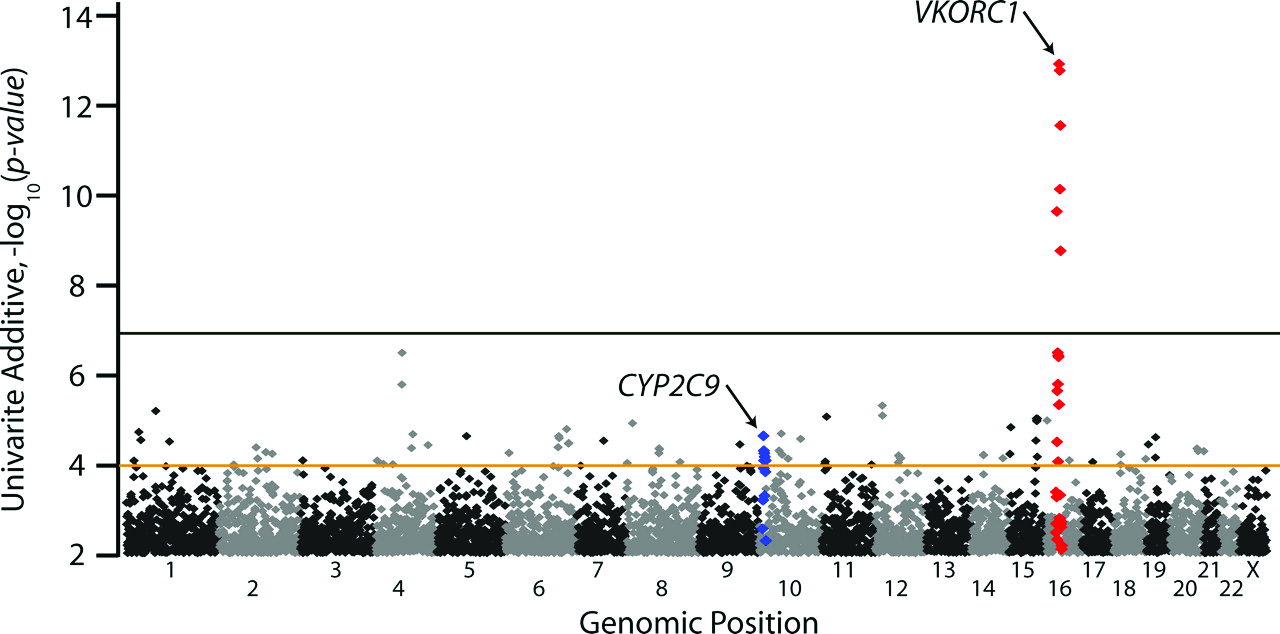
Shortly after World War II, warfarin was introduced for use as a a rat poison. By the mid-1950s it was approved for medical use in the United States as a treatment for diseases in which blood clotting caused a significant threat of stroke. It is still in common use as a treatment for atrial fibrillation.7 Currently, determining the appropriate dose is done by closely monitoring the degree of anticoagulation, an INR of \(2.5 \pm 0.5\) (https://www.drugs.com/dosage/warfarin.html). In an effort to identify genetic markers that could be used to choose an appropriate dosage, investigators at the University of Washington studied the relationship between the dose of warfarin patients were receiving and their genotype at 550,000 SNP loci .8 They identified two loci, VKORC1 and CYP2C9, that were consistently associated with warfarin dose. VKORC1 encodes the vitamin K epoxide reductaxe complex 1 enzyme, and CYP2C9 encodes a cytochrome P450 (Figure 1). Differences at VKORC1 account for approximately 25% of the variance in stabilized dose.9
The GWAS approach I just described works well if the trait we’re studying is continuous,10 but what do we do if the trait we’re interested occurs in only two states, e.g., diseased vs. healthy? Let’s suppose we have a set of “candidate” loci, i.e., loci that we have some reason to suspect might be related to expression of the trait. Now let’s suppose we divide our population sample into two different sets: the “cases,” i.e., those that have the disease,11 and the “controls,” i.e., those that don’t have the disease. Let’s further assume that each of our candidate loci has only two alleles.12 Then for each of our candidate loci we can estimate the allele frequency for the population of cases, \(p_{case}\), and for the population of controls, \(p_{control}\). Then we simply ask, do we have evidence that \(p_{case}\) is different from \(p_{control}\). If so, we have evidence that allelic differences at this locus are associated with different probabilities of falling into the case category, i.e., allelic differences at this locus are associated with a gene that influences development of the phenotype. As with our GWAS analysis, we have to be careful in interpreting this association. It might reflect physical linkage between the candidate locus and the gene influencing phenotypic development or it might reflect nothing more than a statistical association.
It’s pretty obvious that if two loci are on the same chromosome and tightly linked, alleles at those loci are likely to be statistically associated with one another, but let’s take a closer look at what being statistically associated means. We’ll see that while tight physical linkage generally implies statistical association, the reverse isn’t true. A statistical association can arise even if the loci are unlinked and independently inherited.
One of the most important properties of a two-locus system is that it is no longer sufficient to talk about allele frequencies alone, even in a population that satisfies all of the assumptions necessary for genotypes to be in Hardy-Weinberg proportions at each locus. To see why consider this. With two loci and two alleles there are four possible gametes:14
| Gamete | \(A_1B_1\) | \(A_1B_2\) | \(A_2B_1\) | \(A_2B_2\) |
| Frequency | \(x_{11}\) | \(x_{12}\) | \(x_{21}\) | \(x_{22}\) |
If alleles are arranged randomly into gametes then, \[\begin{aligned} x_{11} &=& p_1p_2 \\ x_{12} &=& p_1q_2 \\ x_{21} &=& q_1p_2 \\ x_{22} &=& q_1q_2 \quad , \end{aligned}\] where \(p_1 = \hbox{freq}(A_1)\) and \(p_2 = \hbox{freq}(A_2)\). But alleles need not be arranged randomly into gametes. They may covary so that when a gamete contains \(A_1\) it is more likely to contain \(B_1\) than a randomly chosen gamete, or they may covary so that a gamete containing \(A_1\) is less likely to contain \(B_1\) than a randomly chosen gamete. This covariance could be the result of the two loci being in close physical association, but as we’ll see in a little bit, it doesn’t have to be. Whenever the alleles covary within gametes \[\begin{aligned} x_{11} &=& p_1p_2 + D \\ x_{12} &=& p_1q_2 - D \\ x_{21} &=& q_1p_2 - D \\ x_{22} &=& q_1q_2 + D \quad , \end{aligned}\] where \(D = x_{11}x_{22} - x_{12}x_{22}\) is known as the gametic disequilibrium.15 When \(D \ne 0\) the alleles within gametes covary, and \(D\) measures statistical association between them. It does not (directly) measure the physical association. Similarly, \(D = 0\) does not imply that the loci are unlinked, only that the alleles at the two loci are arranged into gametes independently of one another.
It probably isn’t obvious why we can get away with only one \(D\) for all of the gamete frequencies. The short answer is:
There are four gametes. That means we need three parameters to describe the four frequencies. \(p_1\) and \(p_2\) are two. \(D\) is the third.
Another way is to do a little algebra to verify that the definition is self-consistent. \[\begin{aligned} D &=& x_{11}x_{22} - x_{12}x_{21} \\ &=& (p_1p_2 + D)(q_1q_2 + D) - (p_1q_2 - D)(q_1p_2 - D) \\ &=& \left(p_1q_1p_2q_2 + D(p_1p_2 + q_1q_2) + D^2\right) \\ && \quad - \left(p_1q_1p_2q_2 - D(p_1q_2 + q_1p_2) + D^2\right) \\ &=& D(p_1p_2 + q_1q_2 + p_1q_2 + q_1p_2) \\ &=& D\left(p_1(p_2 + q_2) + q_1(q_2 + p_2)\right) \\ &=& D(p_1 + q_1) \\ &=& D \quad. \end{aligned}\]
In the absence of mutation, \(D\) will eventually decay to 0, although the course of that decay isn’t as regular as what is shown in the Appendix . If we allow recurrent mutation at both loci, however, where \[\begin{array}{ccccccc} &\mu_1 & & & &\mu_2 \\ A_1 &\rightleftharpoons& A_2 &\qquad& B_1 &\rightleftharpoons& B_2 \quad , \\ &\nu_1 & & & &\nu_2 \end{array}\] then it can be shown that the expected value of \(D^2/p_1(1-p_1)p_2(1-p_2)\) is \[\begin{aligned} \frac{\mbox{E}(D^2)}{\mbox{E}(p_1(1-p_1)p_2(1-p_2))} &=& \frac{1}{3 + 4N_e(r+\mu_1+\nu_1+\mu_2+\nu_2) - \frac{2}{(2.5 + N_e(r+\mu_1+\nu_1+\mu_2+\nu_2) + N_e(\mu_1+\nu_1+\mu_2+\nu_2))}} \\ &\approx& \frac{1}{3 + 4N_er} \quad . \end{aligned}\] Bottom line: In a finite population, we don’t expect \(D\) to go to 0, and the magnitude of \(D^2\) is inversely related to amount of recombination between the two loci. The less recombination there is between two loci, i.e., the smaller \(r\) is, the larger the value of \(D^2\) we expect.
This has all been a long way16 of showing that our initial intuition is correct. If we can detect a statistical association between a marker locus and a phenotypic trait, it suggests that the marker locus and a locus influence expression of the trait are physically linked. But we have to account for the effect of population structure, and we have to account for the effect of past population structure.17 Notice also that if the effective population size is large, \(D^2\) may be very small unless \(r\) is very small, meaning that you may need to have a very dense genetic map to detect any association between any of your marker loci and loci that influence the trait you’re studying. As shown in the Appendix, it takes a while for the statistical association between loci to decay after two distinct populations mix. So if we are dealing with populations having a history of hybridization, teasing apart physical linkage and statistical association can become very challenging.18
You can probably guess where this is going. With one locus I showed you that there’s a deficiency of heterozygotes in a combined sample even if there’s random mating within all populations of which the sample is composed. The two-locus analog is that you can have gametic disequilibrium in your combined sample even if the gametic disequilibrium is zero in all of your constituent populations. Table 1 provides a simple numerical example involving just two populations in which the combined sample has equal proportions from each population.
| Gamete frequencies | Allele frequencies | ||||||
| Population | \(A_1B_1\) | \(A_1B_2\) | \(A_2B_1\) | \(A_2B_2\) | \(p_{i1}\) | \(p_{i2}\) | \(D\) |
| 1 | 0.24 | 0.36 | 0.16 | 0.24 | 0.60 | 0.40 | 0.00 |
| 2 | 0.14 | 0.56 | 0.06 | 0.24 | 0.70 | 0.20 | 0.00 |
| Combined | 0.19 | 0.46 | 0.11 | 0.24 | 0.65 | 0.30 | -0.005 |
You knew that I wouldn’t be satisfied with a numerical example, didn’t you? You knew there had to be some algebra coming, right? Well, here it is. Let \[\begin{aligned} D_i &=& x_{11,i} - p_{1i}p_{2i} \\ D_t &=& \bar x_{11} - \bar p_1\bar p_2 \quad , \end{aligned}\] where \(\bar x_{11} = \frac{1}{K} \sum_{k=1}^K x_{11,k}\), \(\bar p_1 = \frac{1}{K} \sum_{k=1}^K p_{1k}\), and \(\bar p_2 = \frac{1}{K} \sum_{k=1}^K p_{2k}\). Given these definitions, we can now calculate \(D_t\). \[\begin{aligned} D_t &=& \bar x_{11} - \bar p_1\bar p_2 \\ &=& \frac{1}{K} \sum_{k=1}^K x_{11,k} - \bar p_1\bar p_2 \\ &=& \frac{1}{K} \sum_{k=1}^K (p_{1k}p_{2k} + D_k) - \bar p_1\bar p_2 \\ &=& \frac{1}{K} \sum_{k=1}^K (p_{1k}p_{2k} - \bar p_1\bar p_2) + \bar D \\ &=& \mbox{Cov}(p_1, p_2) + \bar D \quad , \end{aligned}\] where \(\mbox{Cov}(p_1, p_2)\) is the covariance in allele frequencies across populations and \(\bar D\) is the mean within-population gametic disequilibrium. Suppose \(D_i = 0\) for all subpopulations. Then \(\bar D = 0\), too (obviously). But that means that \[\begin{aligned} D_t &=& \hbox{Cov}(p_1, p_2) \quad . \end{aligned}\] So if allele frequencies covary across populations, i.e., \(\mbox{Cov}(p_1, p_2) \ne 0\), then there will be non-random association of alleles into gametes in the sample, i.e., \(D_t \ne 0\), even if there is random association alleles into gametes within each population.19
Returning to the example in Table 1 \[\begin{aligned} \mbox{Cov}(p_1, p_2) &=& 0.5(0.6-0.65)(0.4-0.3) + 0.5(0.7-0.65)(0.2-0.3) \\ &=& -0.005 \\ \bar x_{11} &=& (0.65)(0.30) - 0.005 \\ &=& 0.19 \\ \bar x_{12} &=& (0.65)(0.7) + 0.005 \\ &=& 0.46 \\ \bar x_{21} &=& (0.35)(0.30) + 0.005 \\ &=& 0.11 \\ \bar x_{22} &=& (0.35)(0.70) - 0.005 \\ &=& 0.24 \quad . \end{aligned}\]
For GWAS this means that we have to be very careful to account for any population structure within our data if we want to interpret a statistical association between a locus and a trait as indicating that the locus is physically associated with a locus influencing expression of the trait. In the example you’ll work through in lab we do this by including an estimate of the genetic relatedness of individuals in our sample in the regression model. Specifically, in this regression equation \[y_i = x_{ij}\beta_j + \phi_i + \epsilon_{ij}\] \(\epsilon\) is pure random error with a mean of 0 and a variance equal to the environmental variance. \(\phi_i\) is a correlated error in which the residual for individual \(i\) is correlated with the residual for individual \(j\) and the degree of correlation is related to the degree of relationship between them.
I’m going to construct a reduced version of a mating table to see how gamete frequencies change from one generation to the next. There are ten different two-locus genotypes (if we distinguish coupling, \(A_1B_1/A_2B_2\), from repulsion, \(A_1B_2/A_2B_1\), heterozygotes as we must for these purposes). So a full mating table would have 100 rows. If we assume all the conditions necessary for genotypes to be in Hardy-Weinberg proportions apply, however, we can get away with just calculating the frequency with which any one genotype will produce a particular gamete.20
| Gametes | |||||
| Genotype | Frequency | \(A_1B_1\) | \(A_1B_2\) | \(A_2B_1\) | \(A_2B_2\) |
| \(A_1B_1/A_1B_1\) | \(x_{11}^2\) | 1 | 0 | 0 | 0 |
| \(A_1B_1/A_1B_2\) | \(2x_{11}x_{12}\) | \(\frac{1}{2}\) | \(\frac{1}{2}\) | 0 | 0 |
| \(A_1B_1/A_2B_1\) | \(2x_{11}x_{21}\) | \(\frac{1}{2}\) | 0 | \(\frac{1}{2}\) | 0 |
| \(A_1B_1/A_2B_2\) | \(2x_{11}x_{22}\) | \(\frac{1-r}{2}\) | \(\frac{r}{2}\) | \(\frac{r}{2}\) | \(\frac{1-r}{2}\) |
| \(A_1B_2/A_1B_2\) | \(x_{12}^2\) | 0 | 1 | 0 | 0 |
| \(A_1B_2/A_2B_1\) | \(2x_{12}x_{21}\) | \(\frac{r}{2}\) | \(\frac{1-r}{2}\) | \(\frac{1-r}{2}\) | \(\frac{r}{2}\) |
| \(A_1B_2/A_2B_2\) | \(2x_{12}x_{22}\) | 0 | \(\frac{1}{2}\) | 0 | \(\frac{1}{2}\) |
| \(A_2B_1/A_2B_1\) | \(x_{21}^2\) | 0 | 0 | 1 | 0 |
| \(A_2B_1/A_2B_2\) | \(2x_{21}x_{22}\) | 0 | 0 | \(\frac{1}{2}\) | \(\frac{1}{2}\) |
| \(A_2B_2/A_2B_2\) | \(x_{22}^2\) | 0 | 0 | 0 | 1 |
Consider the coupling double heterozygote, \(A_1B_1/A_2B_2\). When recombination doesn’t happen, \(A_1B_1\) and \(A_2B_2\) occur in equal frequency (\(1/2\)), and \(A_1B_2\) and \(A_2B_1\) don’t occur at all. When recombination happens, the four possible gametes occur in equal frequency (\(1/4\)). So the recombination frequency,21 \(r\), is half the crossover frequency,22 \(c\), i.e., \(r = c/2\). Now the results of crossing over can be expressed in this table:
| Frequency | \(A_1B_1\) | \(A_1B_2\) | \(A_2B_1\) | \(A_2B_2\) |
|---|---|---|---|---|
| \(1-c\) | \(\frac{1}{2}\) | 0 | 0 | \(\frac{1}{2}\) |
| \(c\) | \(\frac{1}{4}\) | \(\frac{1}{4}\) | \(\frac{1}{4}\) | \(\frac{1}{4}\) |
| Total | \(\frac{2-c}{4}\) | \(\frac{c}{4}\) | \(\frac{c}{4}\) | \(\frac{2-c}{4}\) |
| \(\frac{1-r}{2}\) | \(\frac{r}{2}\) | \(\frac{r}{2}\) | \(\frac{1-r}{2}\) |
We can use the mating table table as we did earlier to calculate the frequency of each gamete in the next generation. Specifically, \[\begin{aligned} x_{11}' &=& x_{11}^2 + x_{11}x_{12} + x_{11}x_{21} + (1-r)x_{11}x_{22} + rx_{12}x_{21} \\ &=& x_{11}(x_{11} + x_{12} + x_{21} + x_{22}) - r(x_{11}x_{22} - x_{12}x_{21}) \\ &=& x_{11} - rD \\ x_{12}' &=& x_{12} + rD \\ x_{21}' &=& x_{21} + rD \\ x_{22}' &=& x_{22} - rD \quad . \end{aligned}\]
We can also calculate the frequencies of \(A_1\) and \(B_1\) after this whole process: \[\begin{aligned} p_1' &=& x_{11}' + x_{12}' \\ &=& x_{11} - rD + x_{12} + rD \\ &=& x_{11} + x_{12} \\ &=& p_1 \\ p_2' &=& p_2 \quad . \end{aligned}\] Since each locus is subject to all of the conditions necessary for Hardy-Weinberg to apply at a single locus, allele frequencies don’t change at either locus. Furthermore, genotype frequencies at each locus will be in Hardy-Weinberg proportions. But the two-locus gamete frequencies change from one generation to the next.
You can probably figure out that \(D\) will eventually become zero, and you can probably even guess that how quickly it becomes zero depends on how frequent recombination is. But I’d be astonished if you could guess exactly how rapidly \(D\) decays as a function of \(r\). It takes a little more algebra, but we can say precisely how rapid the decay will be. \[\begin{aligned} D' &=& x_{11}'x_{22}' - x_{12}'x_{21}' \\ &=& (x_{11} - rD)(x_{22} - rD) - (x_{12} + rD)(x_{21} + rD) \\ &=& x_{11}x_{22} - rD(x_{11} + x_{12}) + r^2D^2 - (x_{12}x_{21} + rD(x_{12} + x_{21}) + r^2D^2) \\ &=& x_{11}x_{22} - x_{12}x_{21} - rD(x_{11} + x_{12} + x_{21} + x_{22}) \\ &=& D - rD \\ &=& D(1-r) \end{aligned}\] Notice that even if loci are unlinked, meaning that \(r = 1/2\), \(D\) does not reach 0 immediately. That state is reached only asymptotically. The two-locus analogue of Hardy-Weinberg is that gamete frequencies will eventually be equal to the product of their constituent allele frequencies.
These notes are licensed under the Creative Commons Attribution License. To view a copy of this license, visit or send a letter to Creative Commons, 559 Nathan Abbott Way, Stanford, California 94305, USA.